
Curly
-
Posts
173 -
Joined
-
Last visited
3 Followers

-
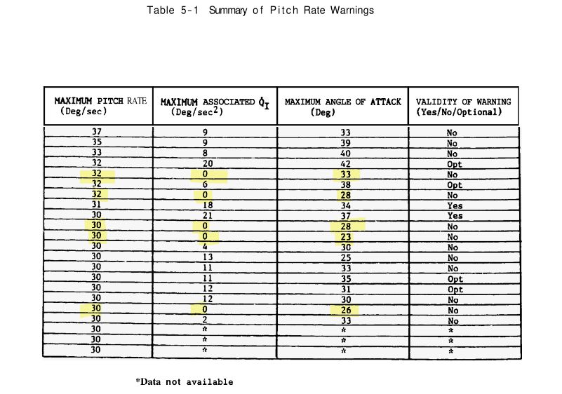
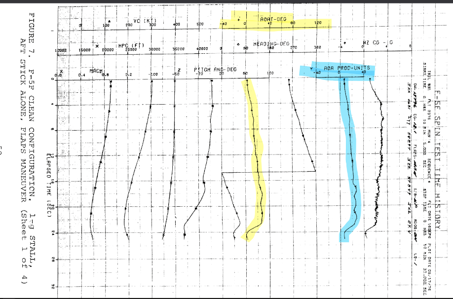
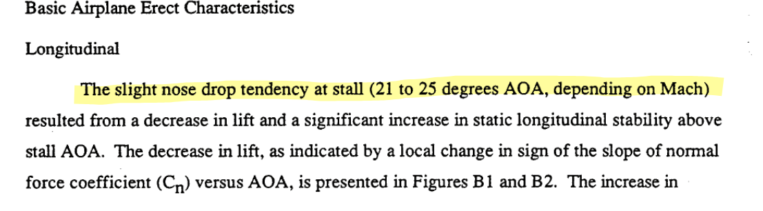
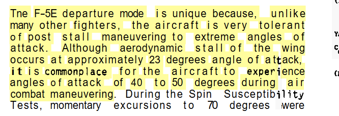
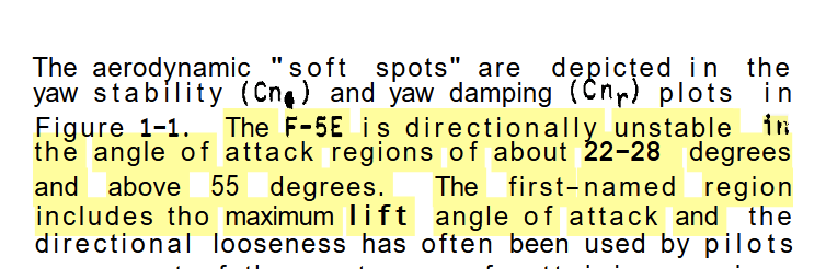
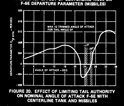
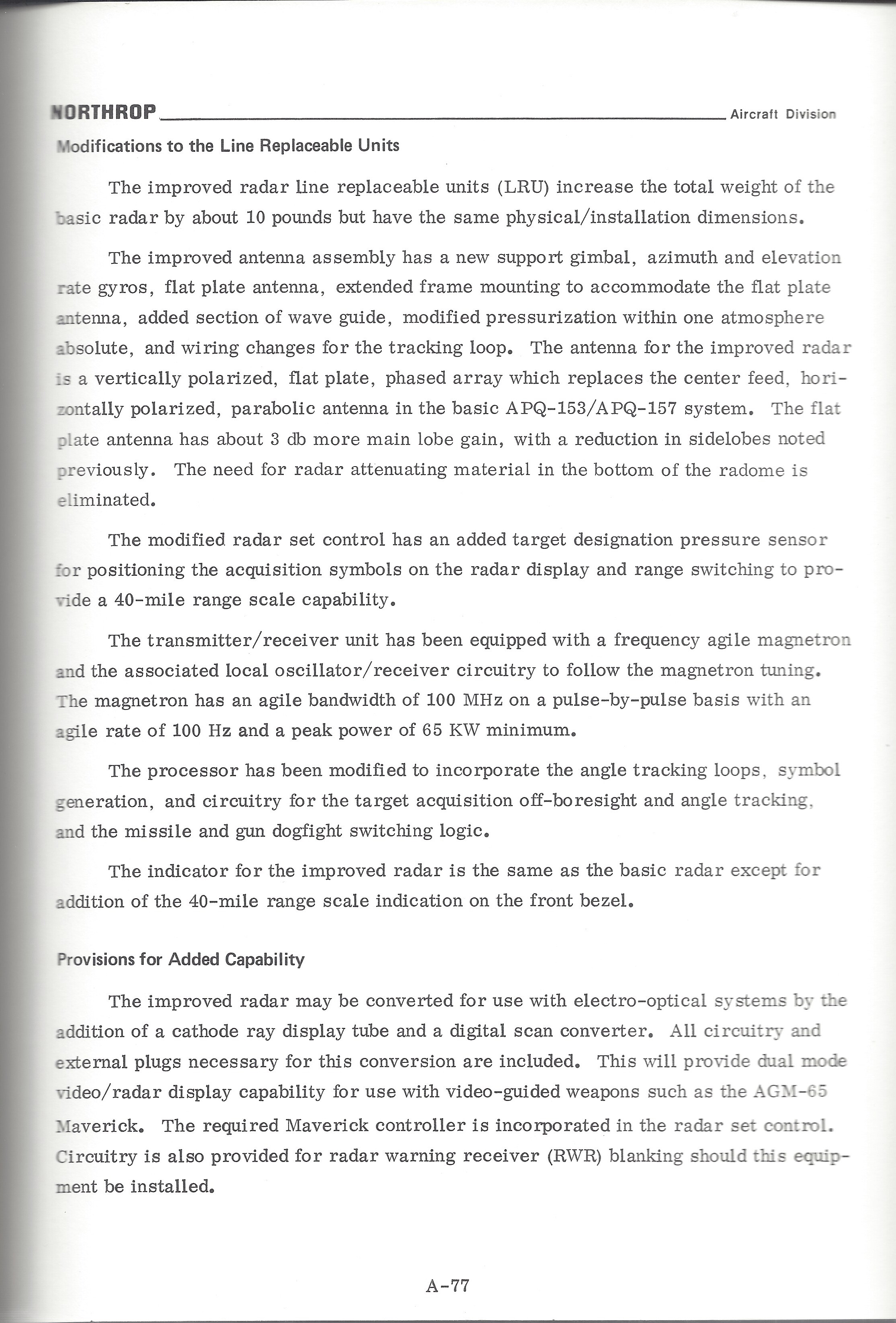
There are 2 distinct conversations going on in this thread, the conversion of AOA units to degrees, along with a discussion about AOA capabilities of the F-5E. First lets briefly touch on the conversion of AOA units to degrees in the F-5E. I have finished scanning the entire Northrop F-5E Technical Description manual and it is now posted on archive.org for free. https://archive.org/details/f-5-e-technical-description This document does not contain a definitive algorithm for converting AOA units to degrees. However, utilizing the description of the Air Data Computer from the F-5E Technical Description, along with additional data from the 1986 version of the Skow and Taylor report “F-5E Departure Warning System Algorithm Development and Validation”, The Air Force AFFTC F-5 Spin Report, And better scan of the NASA Shark Nose Report. it is possible to make a good approximation of the relationship between AOA units and degrees. Based on my evaluation of the source material, I would estimate that AOA units = AOA true in degrees * 1.1 The data and procedures used to determine this value will be provided below. Following a brief discussion of stall and max AOA’s of the F-5E. Briefly, the max AOA that is possible in the F-5E is dynamic and dependent on pitch rates, inertial coupling, and aircraft configuration. In the 1986 version of the Skow Departure Warning System paper. https://arc.aiaa.org/doi/abs/10.2514/6.1986-2284 There is a table of Maximum AOA’s, the pitch rates, and the pitch acceleration due to inertial coupling. The data was taken from F-5E flight tests and air combat training. The aircraft were configured with the CG at 18.5 to 19.0 % of the Mean aerodynamic chord. Examination of the max AOA’s obtained without inertial coupling, indicated that pitch rates greater than 30 degrees per second might be required to achieve AOA’s greater than 21 to 25 degrees. Lets now return to the issues of converting AOA units to degrees in the F-5E. As stated previously my estimate for AOA conversion factor is. AOA units = AOA true in degrees * 1.1 It is based on the description of the central air data computer, CADC, contained in the Northrop F-5E/F Technical Description. One of the key functions of the CADC is to convert Indicated AOA to True AOA for the gunsight system. <iframe src="https://archive.org/embed/f-5-e-technical-description" width="560" height="384" frameborder="0" webkitallowfullscreen="true" mozallowfullscreen="true" allowfullscreen></iframe> https://archive.org/details/f-5-e-technical-description/page/4-111/mode/1up The CADC provides True AOA to gunsight from -4 to 29 degrees, thus True AOA is reported over a range of 33 degrees as, 4 + 29 = 33 The system is accurate to +-1 degree over the range -2 to + 24 degrees. Therefore the system is accurate over a range of 26 degrees. Indicated AOA is reported from 0 to 30 Units., a range of 30 units. Let's put these values in a table to clarify. AOA Units AOA True AOA Accurate max 30 29 24 min 0 -4 -2 Range 30 33 26 Lets begin by asking if we can even assume that the relationship between AOA units and degrees is even linear in a 1g stick aft stall. I managed to acquire a physical copy of the NASA Shark Nose report and created a high quality scan of some of the flight test data. To my surprise the F-5F 1 g stall test data actually does contain a record of AOA true in degrees and AOA units. The relationship between units and degrees does appear to be linear in these tests. Which means that converting AOA units to degrees may be as simple as dividing either 33 / 30 or 26 /30. The description of the CADC gives two ranges over which AOA true is computed for the gunsight. The range in which the system is accurate to +-1 degree, we’ll call the AOA Accurate and the larger range between 29 and -4 degrees, well call AOA True. Now must decide which calibration, Accurate or True is correct. To determine the correct AOA conversion factor, we will convert AOA data from the flight manuals and test with both calibrations, Accurate and True. Then pick the most reasonable fit. AOA Units AOA true AOA Accurate max 30 29 24 min 0 -4 -2 Range 30 33 26 Deg to Units 1.1 0.866 The F-5E pilots manual states that the AOA for on speed for the landing approach is 15.8 units indicated on the dial. Lets determine the Approach AOA in degrees AOA Units AOA true AOA Accurate max 30 29 24 min 0 -4 -2 Range 30 33 26 Deg to Units 1.1 0.866 Units to Degs 1 /1.1 1 /0.8666 Approach AOA 15.8 14.36 18.23 AOA True predicts the approach AOA is 14.36 degrees. AOA Accurate predicts the approach AOA is 18.23 degrees. Now let's look at some data from the F-5E flight manual. The flight manual notes that the stall AOA for the early F-5E’s is 24 units. Lets compute the stall AOA for the Early F-5E. AOA Units AOA true AOA Accurate max 30 29 24 min 0 -4 -2 Range 30 33 26 Deg to Units 1.1 0.866 Units to Degs 1 /1.1 1 /0.8666 Approach AOA 15.8 14.36 18.23 Early FM 24 21.8 27.69 AOA True predicts the stall AOA to be, 21.8 Degrees. AOA Accurate predicts the stall AOA to be, 27.69 Let's compare the computed stall AOA’s to stall AOA from some flight tests. An extract from the Air Force’s F-5E/F Spin Report , gives the stall AOA as 21 to 25 degrees. See Pages 146 and 147. https://apps.dtic.mil/sti/pdfs/ADA319981.pdf The conversion factor AOA True ( AOA units = AOA degrees * 1.1) seems to be more accurate. As it closely matches the results of the Air Force Flights. AOA Units AOA true AOA Accurate max 30 29 24 min 0 -4 -2 Range 30 33 26 Deg to Units 1.1 0.866 Units to Degs 1 /1.1 1 /0.8666 Approach AOA 15.8 14.36 18.23 Early FM 24 21.8 27.69 Air Force 21 In The 1986 version of Skow’s Departure Warning System report. The aerodynamic stall AOA is given as 23 degrees. He also notes that the F-5E becomes directionally stable at 22-28 degrees AOA, referring to this area as the departure window. In tabular data, the largest AOA achieved without pitch coupling was 33 degrees. Skow is also the one of the authors of the report “Design of Technology for Departure Resistance of Fighter Aircraft” from the AGARD conference paper often cited here. He gives the Max 1 G trimmed AOA of an F-5E with missiles and a center fuel tanks as 24 degrees. It should be noted that the max trim AOA is not the same as the maximum or stall AOA. Max Trim AOA is the largest steady state AOA that can be with the flight controls. Let’s take all these data points along with the stall AOA from the Air Force report, put them into a table and convert from degrees to units. AOA Skow AOA True AOA Accurate Degrees Units Units Stall 23 25.3 19.9 Departure 22 24.2 19.1 Trim AOA 24 26.4 20.8 Max AOA 33 36.3 28.6 Air Force Stall 21 23.1 18.2 We’ll conclude the analysis by returning to the pilots manual and examining the auto flap system on the F-5E3. The maneuvering flap schedule is based on indicated AOA. The position of flaps changes with indicated AOA and the air speed. Up to 330 KIAS the flap position changes at 13.6, 12, 10 and finally at 7.5 units of AOA. The aircraft Stalls at 27 to 28 units of AOA, buffet on begins at 15 to 17 Units of AOA. If the stick is held full to 30 AOA The Aircraft will drop a wing depart AOA Units AOA true deg AOA Acc deg Skow AOA Deg Depart 30 27.3 34.6 22 Buffet 17 15.5 19.6 Stall 27 24.5 31.2 23 Stall 28 25.5 32.3 Flap Max 13.6 12.4 15.7 Flap Mid 12 10.9 13.8 Flap Mid 1 10.1 9.1 11.5 Flap Lo 7.5 6.8 8.7 I’ll probably make being making an export script and use most of this information later.

-
investigating Aileron Spring Stop / Aileron Limiter
Curly replied to Curly's topic in Bugs and Problems
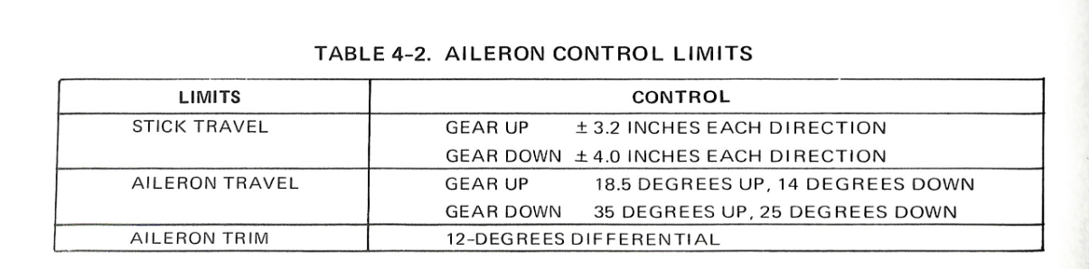
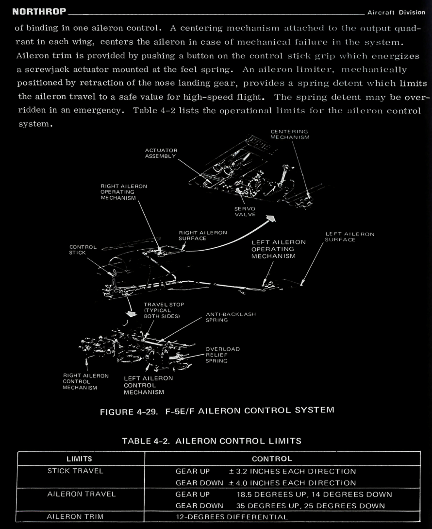
Sure, First lets clarify what is exactly stated in the flight manual about the aileron limiter. The flight manual states that full Aileron travel is 35 Degrees Up 25 Degrees Down. The manual also states that the spring stop limits AILERON TRAVEL to 1/2. The Flight manual does not state that the control stick is limited to half of its travel when the spring stop is engaged. The description of the aileron flight controls from the Northrop F-5/E Technical Description proves that the aileron limiter is physically located at 80% of the control sticks travel. This document contains the Stick Travel Limits, and the aileron travel limits. When the Landing Gear is down: The aileron limiter is turned off. And Full Aileron Travel is available, (35 up / 25 down), and Full Stick Travel to 4 inch is available. When The Landing Gear is UP, The aileron limiter is on. Aileron Travel is Limited to 18.5 Up / 14 Down, Stick Travel is Limited to 3.2 Inches. Thus when the Aileron limiter is active. The Stick travel is limited to 80% as (3.2 / 4) = 0.8 And Aileron travel is limited to 50 % as (18.5 / 35) = 0.52 Thus, the Aileron Limiter / Spring Stop is physically located at 80% of the sticks travel (3.2 inches) and limits aileron travel to 50%. As described in the pilots manual. If the stick is limited to 3.2 inches and the aileron 18.5 degrees, than limiter can only be located at 80% of the stick travel.
-
investigating Aileron Spring Stop / Aileron Limiter
Curly replied to Curly's topic in Bugs and Problems
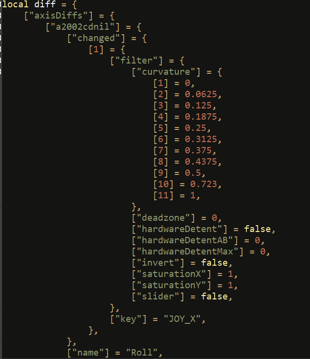
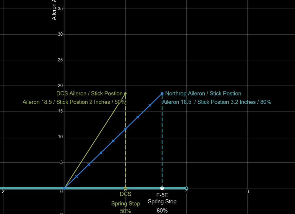
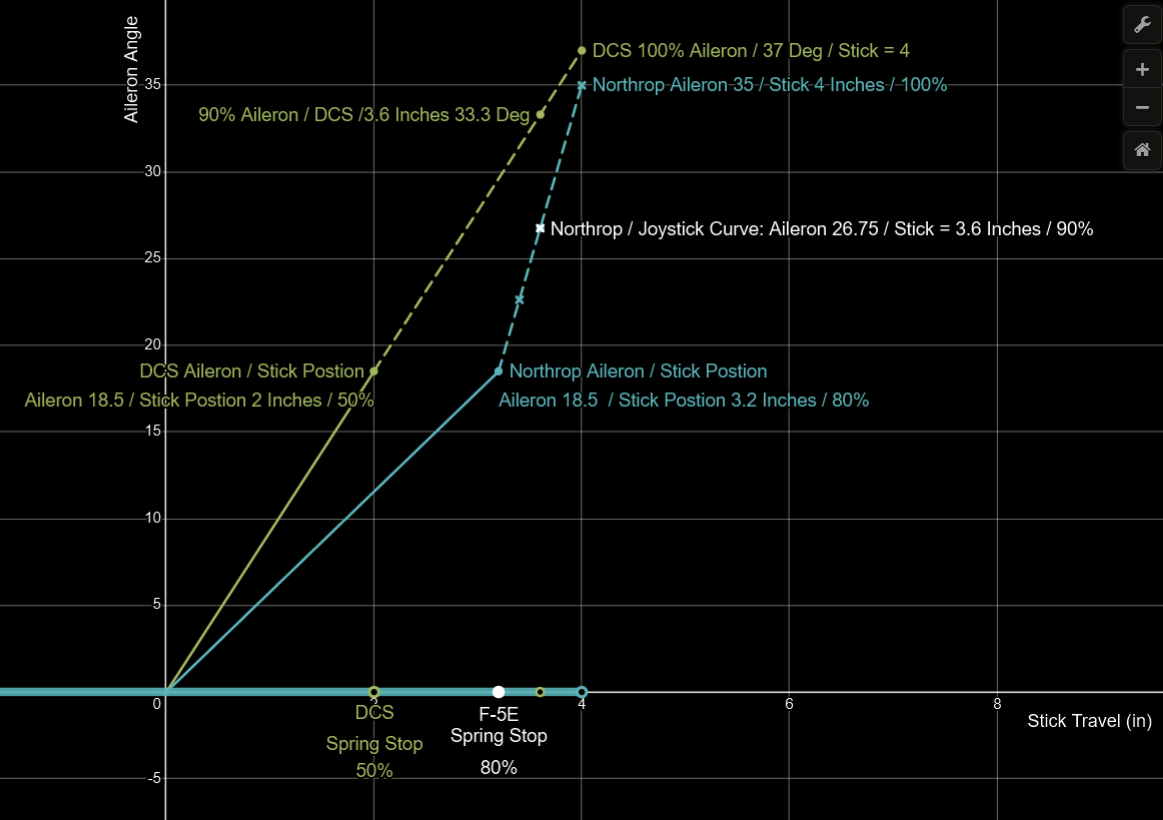
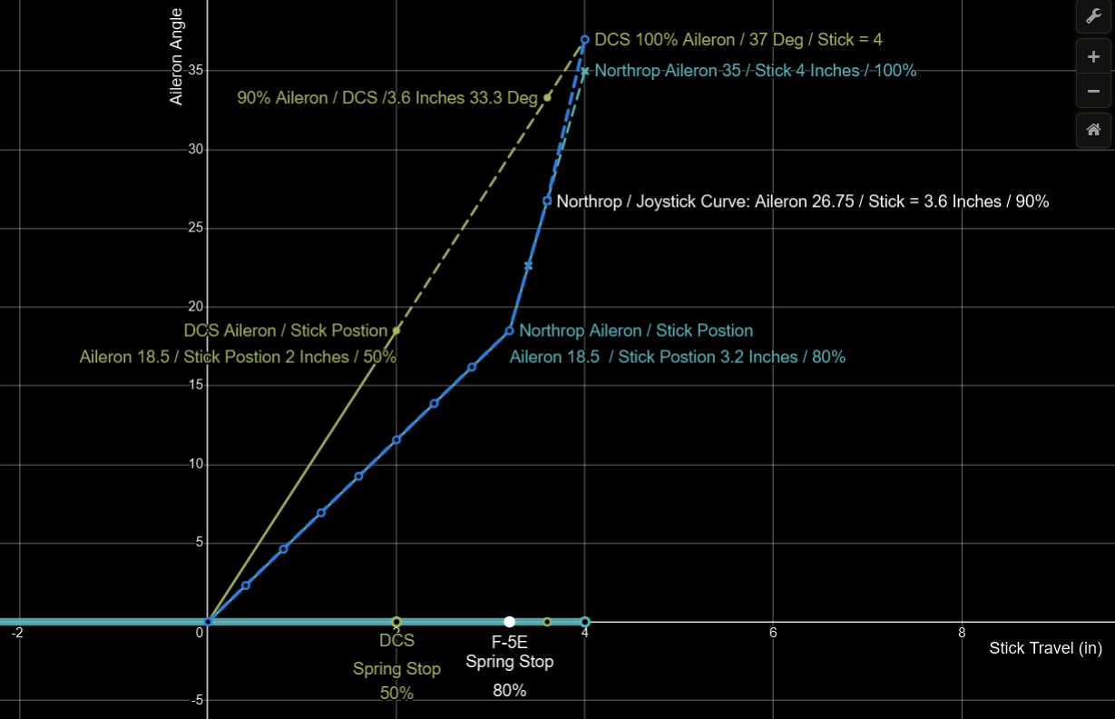
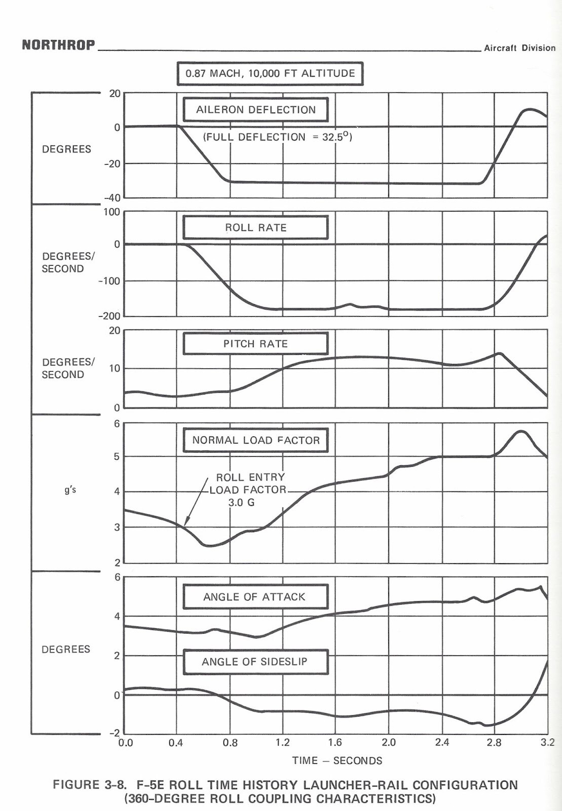
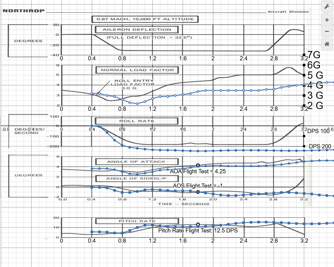
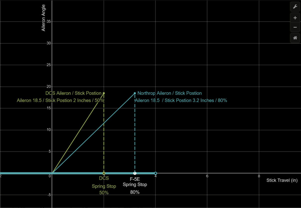
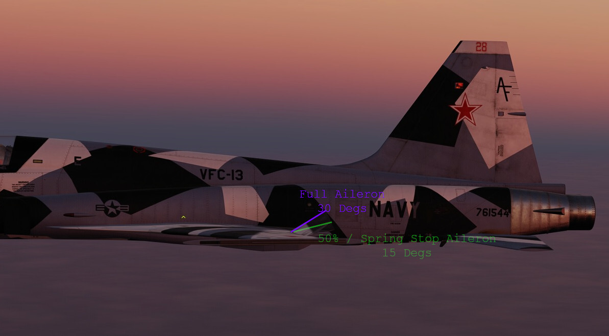
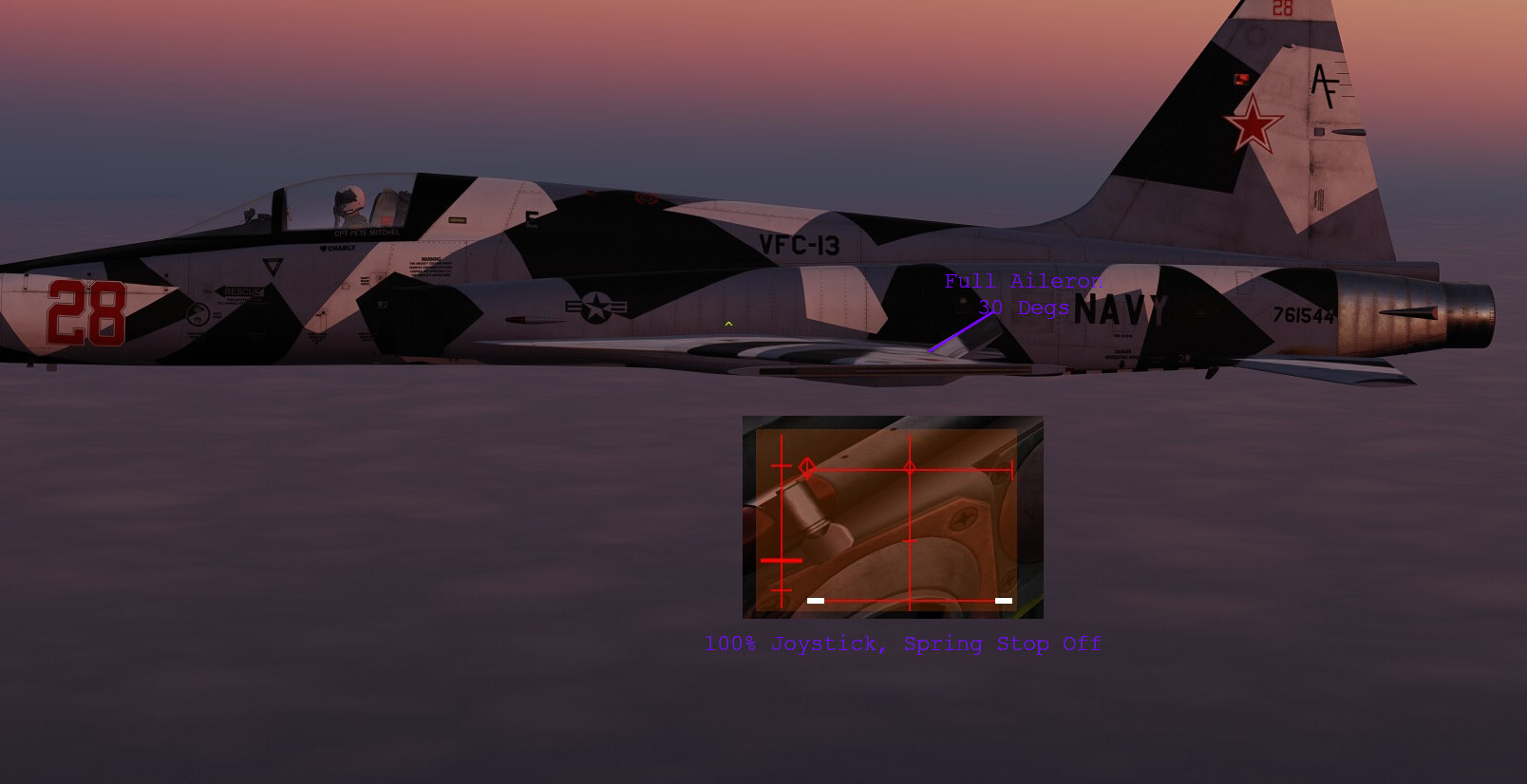
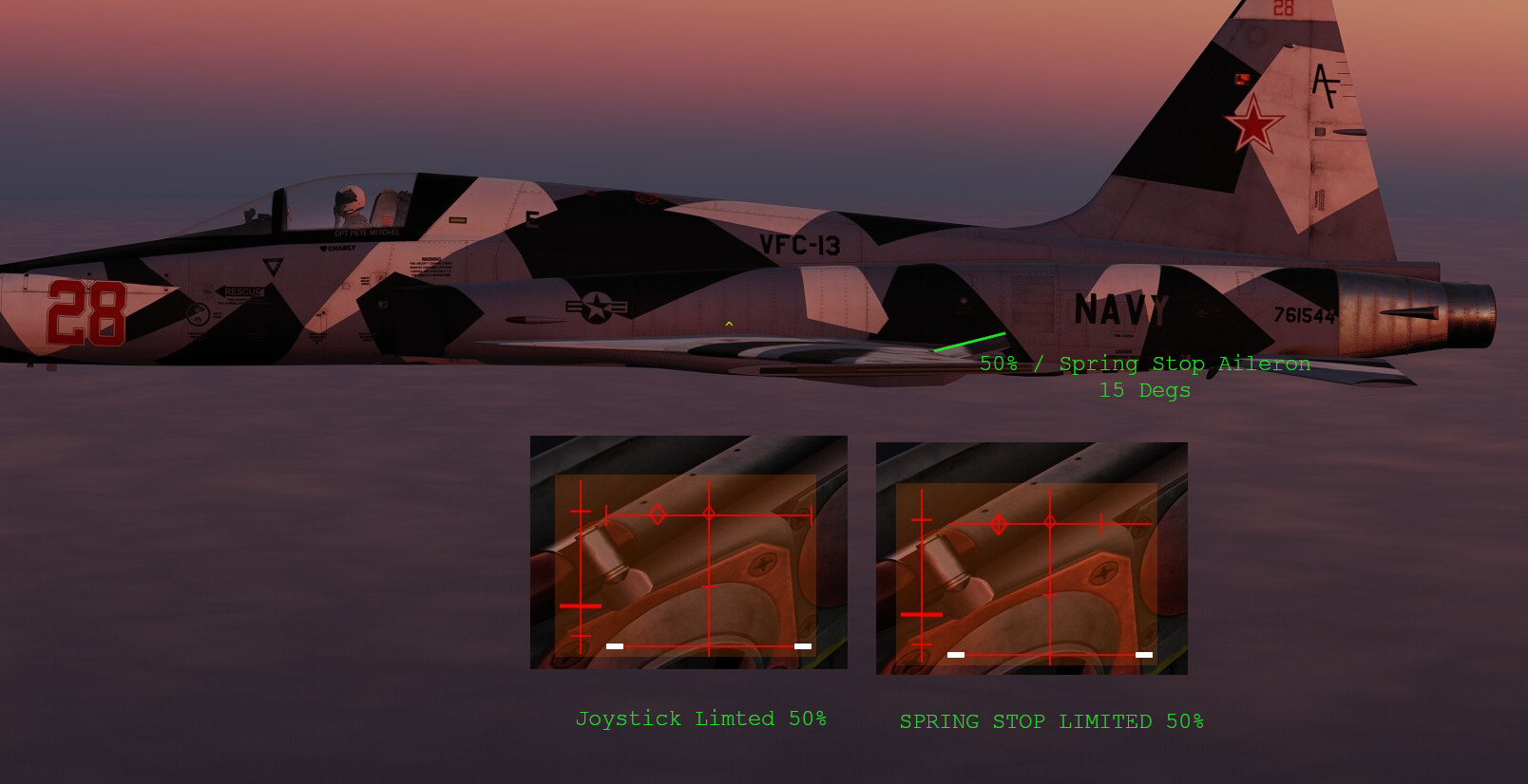
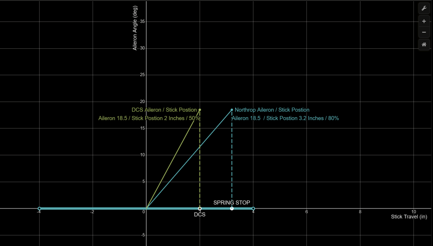
In order to match the lateral (roll) handling qualities of the real F-5E. I have created a custom joystick curve which transforms the aileron gearing ratio (aileron angle / control stick) of the DCS F-5E to match the real aircraft as closely as possible. The realistic / custom axis curve results in improved precision without reducing roll rate performance. I would recommend that this custom roll axis curve be implemented in the nonlinear joystick axis settings of the DCS F-5E, as it is historically accurate. The roll axis curve as implemented in DCS. Was based on information from the Northrop Technical Description and from flight testing the DCS F-5E . Which has been previously presented. Based upon this data we know that the Aileron Limiter / Spring stop in DCS is located at 50 % joystick output. While in the real aircraft, the Spring Stop is located at 80 % of the Stick travel, 3.2 Inches) Lets plot and compare the ratio of the aileron angle to stick deflection of the real aircraft and the DCS F-5E. From 0 stick deflection to the Spring Stop. The custom roll axis curve presented above will move the DCS Aileron Limiter / Spring Stop to 80% of the joystick travel and match the linear slope of the gearing ratio to the spring stop. This was achieved by multiplying the output of DCS joystick axis by 0.625 for the first 80 % of the joystick output. As 0.625 is = (The F-5E Aileron Gearing Ratio (18.5 / 3.2) / The Gearing Ratio of the DCS F-5 (18.5 / 2) The custom roll axis curve also closely matches the aileron gearing ratio when the control stick is pushed beyond the spring stop. Let compare the aileron gearing ratio of the DCS F-5E and Northrop F-5E when the control stick is moved pasted the spring stop Note that the aileron gearing ratio of the DCS F-5E is the same across the entire range of control stick deflection. At 100 % stick input we could assume the max aileron angle of the DCS F-5E is about 37 Degrees trailing edge up. And at 90% Stick input the aileron angle is 33.3 degrees. In the real aircraft the aileron gearing ratio increases when the control stick is moved past the spring stop. At 100% stick input (4 inches) the aileron angle is 35 degrees. And at 90 Stick input, the aileron angle is 26.75 degrees. To best match the real Aileron gearing with our custom DCS joystick Curve. We'll adjust the joystick output at 90 % to match the Northrop data. We need to reduce the output of the joystick axis from 33.33 to 26.75. We also need to keep in mind that the max aileron angle of the DCS F-5E is 37 degrees. In order to best fit the Real Curve we should Reduce the Stickout put by 72.3%, as 37*0.723 = 26.57 The purposed custom roll axis curves, depicted in blue below, results in a nearly identical aileron gearing ratio, when compared to the real aircraft The improved aileron gearing ratio below the spring stop. improves the flying qualities of the DCS F-5E by making it less sensitive, which improves fine tracking and bank angle control. Comparing Northrop F-5E Roll Rate Flight Test from the Technical Description: To DCS F-5E roll rate tests conducted under the same conditions with custom axis curve implemented. Indicate similar roll rate performance. https://www.desmos.com/calculator/fd1tis4pnk I've also attached my Joystick Config file with custom axis curve. I high recommend using a txt editor like notepadd ++ to implement this curve on other joysticks. As you can not use decimal places within the DCS custom curve tool. null F-5E Warthog Stick With Curve_2.diff.lua
-
investigating Aileron Spring Stop / Aileron Limiter
Curly replied to Curly's topic in Bugs and Problems
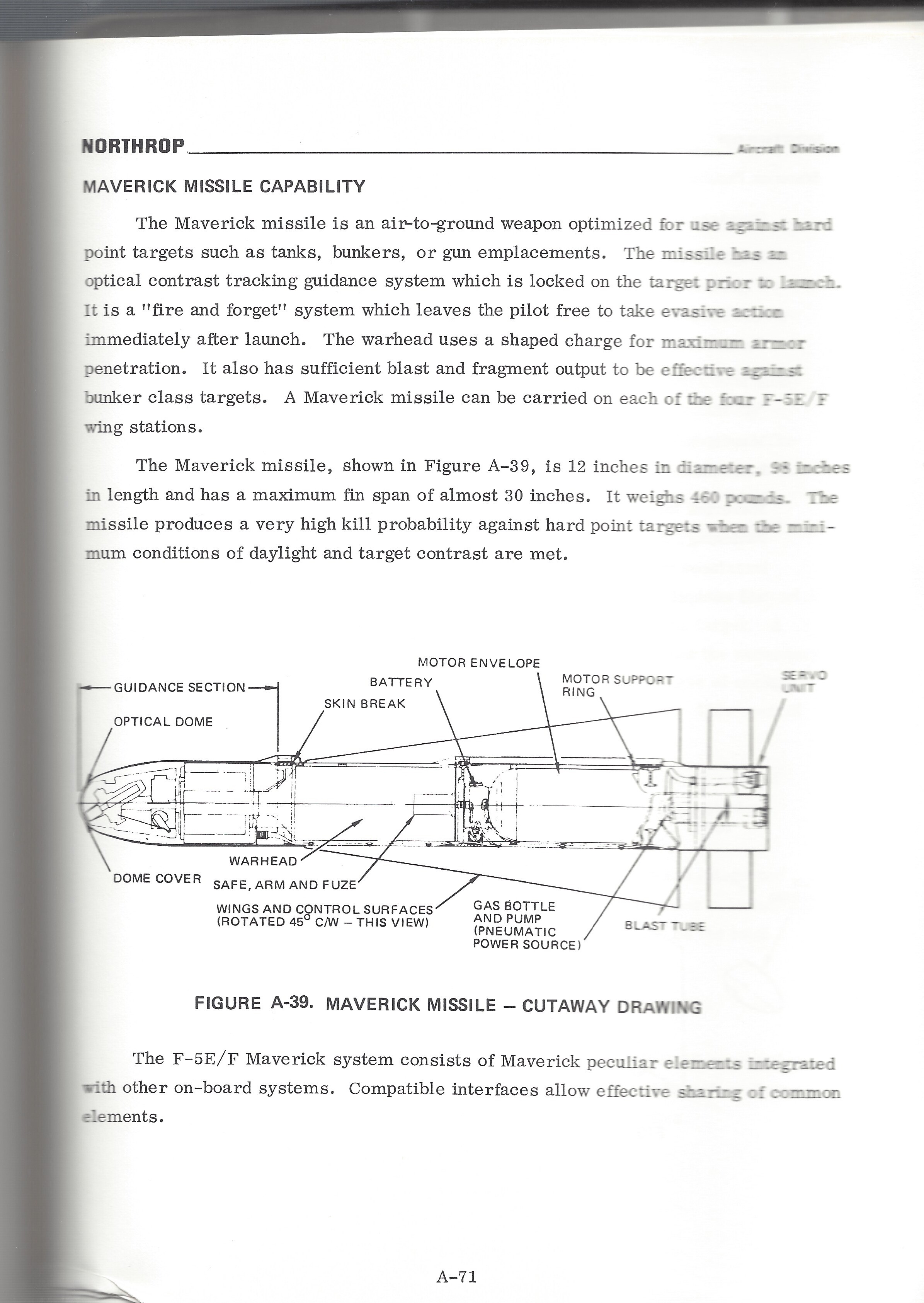
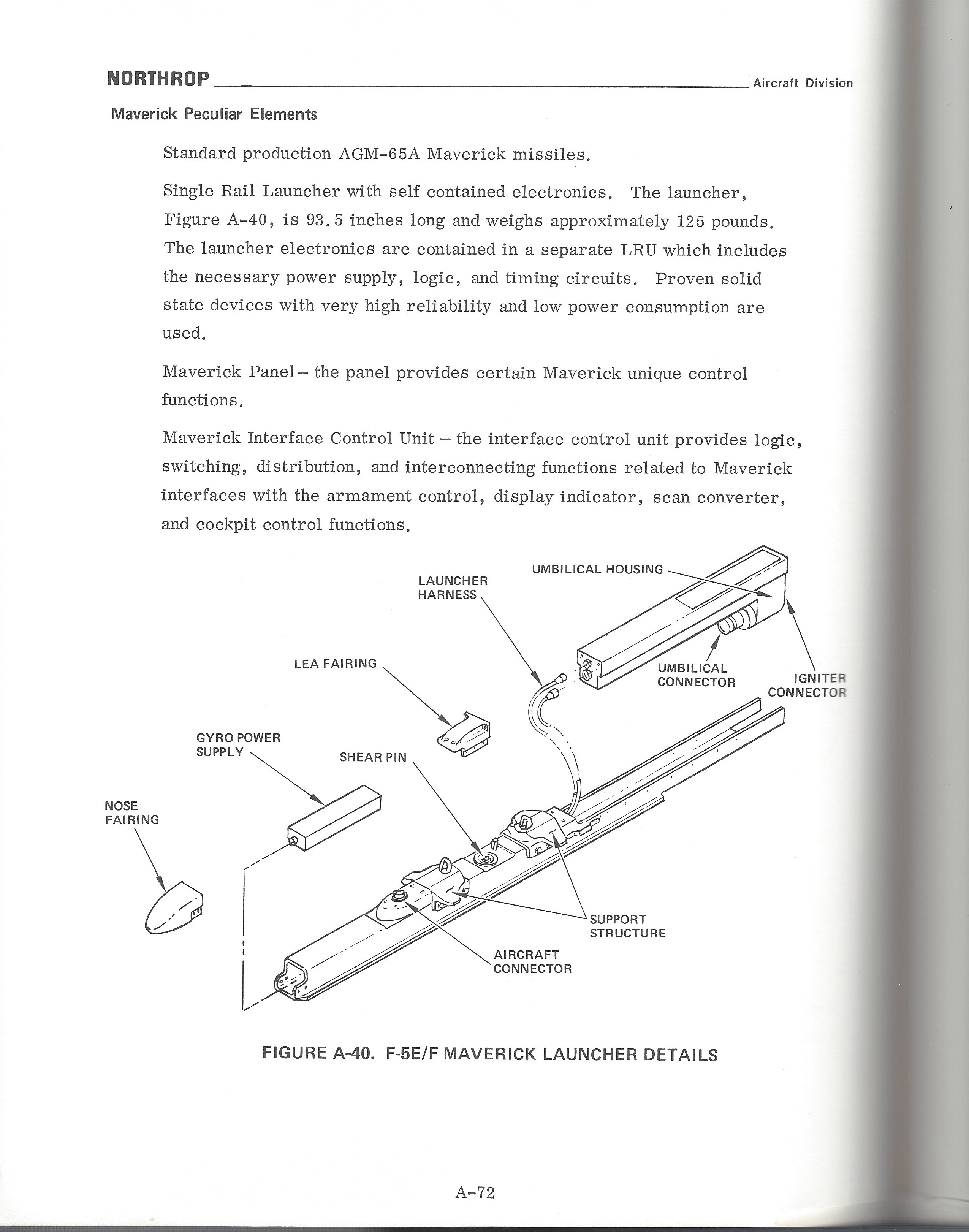
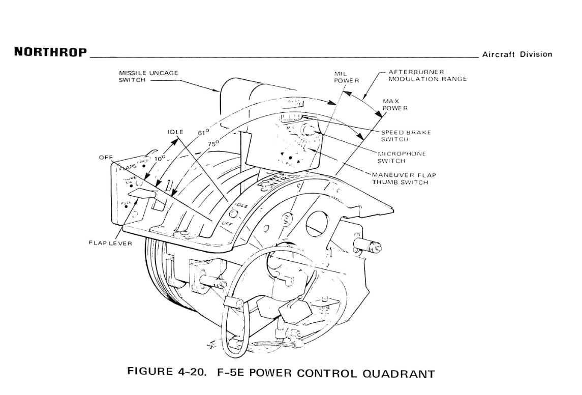
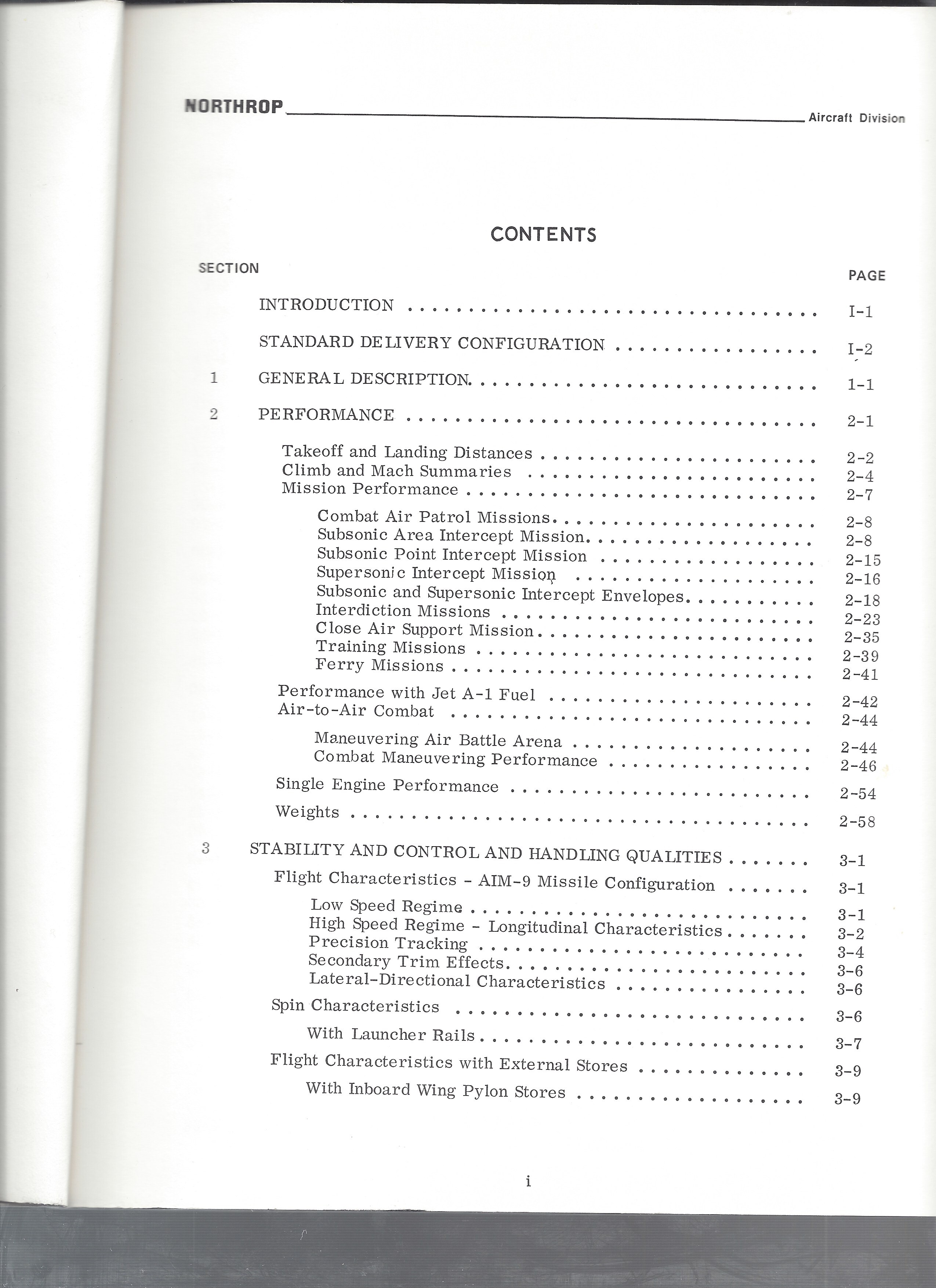
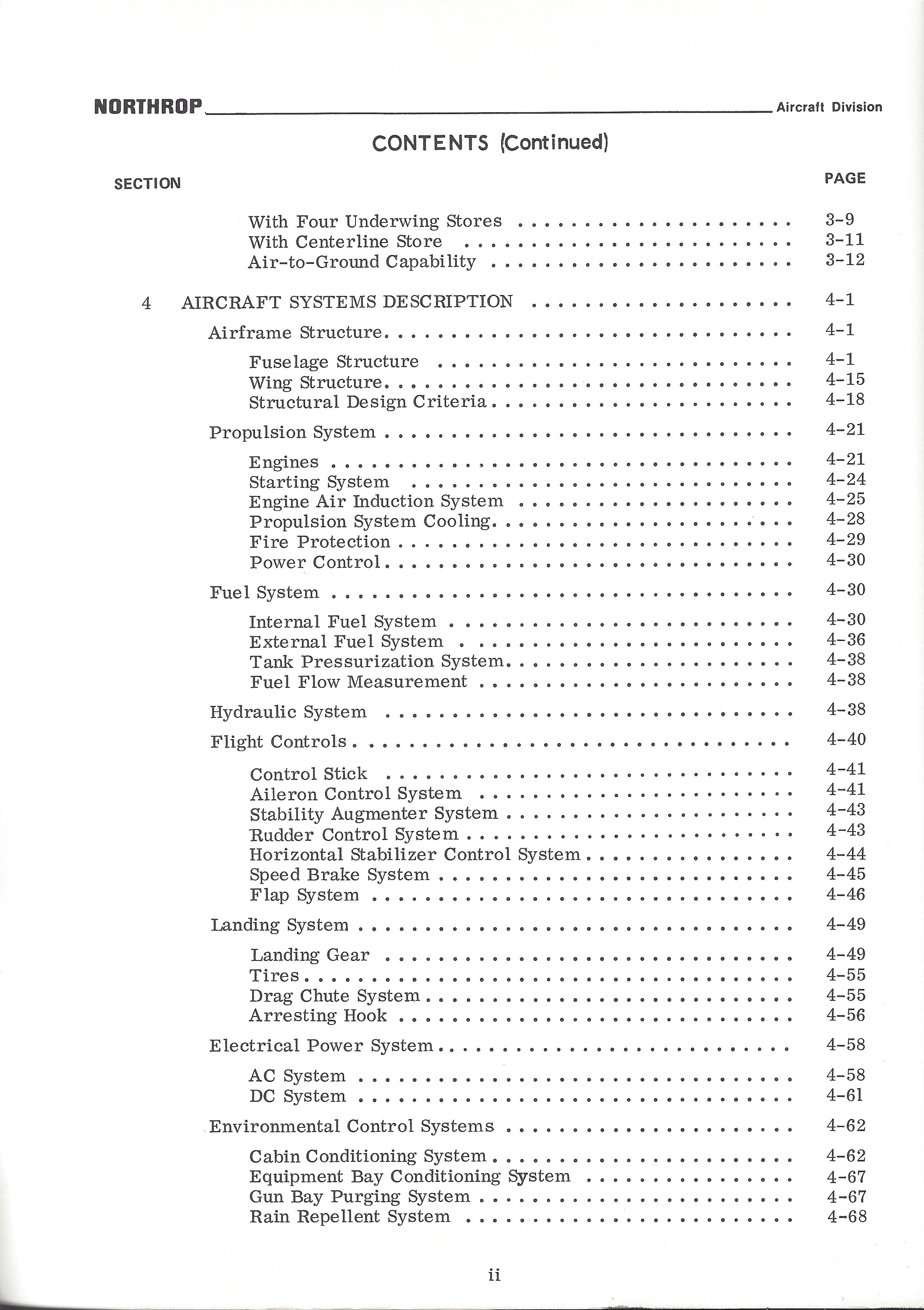
Hey I'm happy to see this post getting some engagement. I was away on vacation last week and unable to respond. I have two physical copies of the Northrop Technical Description of the F-5E/F from different dates. I got the both from Ebay Both reports have the same Northrop Report number NB 74-36, but with different revision dates. The cover to the report posted above is from 1975 version. I also have a copy the 1976 version of this manual. It contains most of the same information as the 1975 version of the same document. The 1975 Version of the document is more interesting as it describes the Air To Air Refuling System: Here's a video of the test pilot describing the flight testing of the Air to Air to refueling system and the problems they encountered. The 1975 Version also describes the planned implementation of the Maverick Missile System: The performance of the APQ-153 radar: And the expected performance of the upgraded fire control which would become know as the APQ-159. There's also a few other details and diagrams, such as the angle of operation of the throttles. That home simpit buliders like @Bucic may find interesting. null I'll post the table of Contents for the 1975 version below. I'm happy to provide scans of sections of the manual upon request. After I upgrade my scanning setup, I'll post a complete scan of both documents. In DCS I have measured the stick deflection Vs aileron angle using active pause and Photoshop. In DCS, At 50% stick Deflection, where the aileron spring stop is located: The aileron angle is equal to half of the maximum. Which indicates that the location of the spring stop (aileron limiter) and the gearing ratio of the aileron angle to control stick input in DCS is inaccurate. The equivalent aileron gearing ratio of the DCS F-5E; 18.5 Degrees of aileron angle, per 2 inches of stick movement (18.5/2). Is 1.6 times greater than the gearing ratio of the real F-5E: 18.5 Degrees of aileron angle per 2 inches of stick movement (18.5/3.2) as (18.5/2) / (18.5 /3.2) = 1.6 Thus, along the roll axis the DCS F-5E is much more sensitive to roll inputs than the Northrop documents indicate.
-
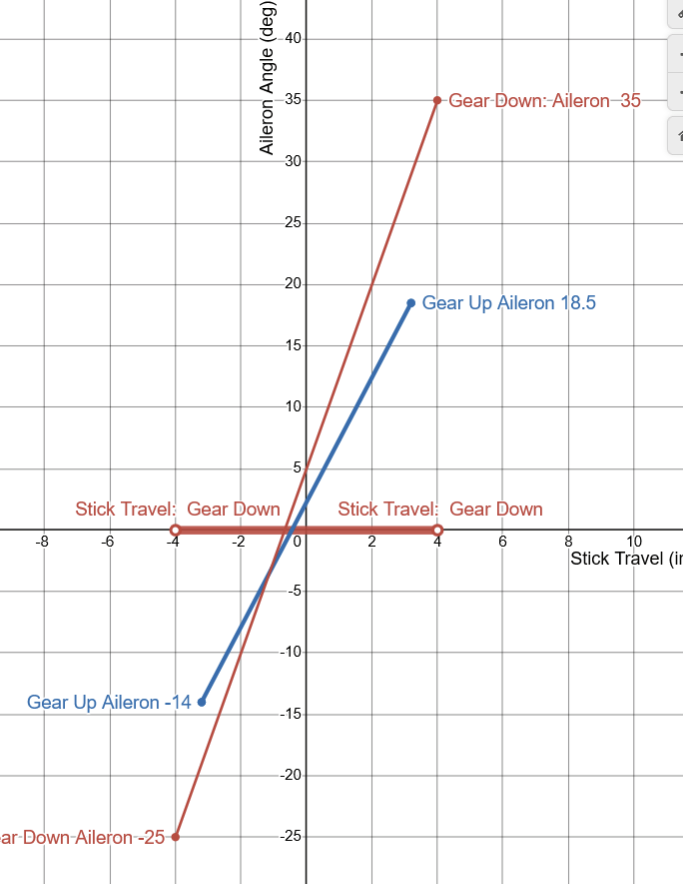
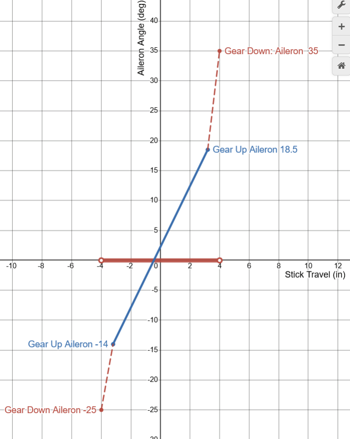
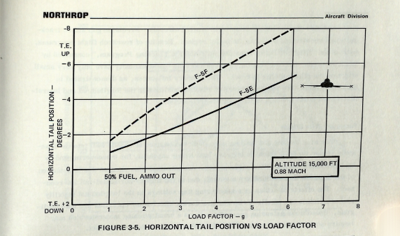
Requested Change: Move the position of the spring stop to 80% of the aileron axis. Problem: On the DCS F-5E, the aileron limiter / the spring stop, is located at 50 % of the aileron axis. Placement of the Spring Stop here is inaccurate and makes the F-5 difficult to accurately control laterally. To be clear, I am not calling for the removal of the spring stop, only that it moved to 80% of the joystick axis. While it is true that the spring stop limits the total aileron deflection by more than 50%, as is stated in the F-5E flight manual: Examination of more detailed descriptions of the flight control contained in official Northrop documentation Indicates that aileron deflection per control stick movement (the aileron gearing) is not linear and that the spring stop should be located at 80% of the roll stick travel. With the landing gear down: Stick Travel is = +- 4.0 inches, and the max aileron angle is 35 degrees Up, 25 degrees Down. For a total Aileron Angle of 60 degrees When the landing gear is up, the aileron limiter / spring stop is active. The Stick Travel is limited to: +- 3.2 inches. Thus the spring stop is located +- 3.2 inches from the center. +-3.2 being equivalent to 80% of the total Stick Travel (4 inches). As (3.2 / 4) = %80 At 80% stick travel; the aileron angle is limited to 18.5 degrees Up, 14 degrees down. The spring stop therefore limits total aileron angle by more than 50%. As (18.5+14) / (35 +25) = 54% While the details of the Northrop Technical Manual match the description of the Aileron Limiter from the Pilots Manual, “Limits the Aileron travel to one half”. Neither sources state that the flight controls are limited to 50% / half travel when the landing gear is raised. Plotting the aileron angles and stick position from the Technical Description, and connecting these points by the appropriate slope. We constructed a diagram depicting the aileron angle as a function of the stick position, often called the aileron gearing ratio. This chart indicates that the aileron limiter in the landing gear up (aileron limited) config, cannot be located at 50% position of the total control stick travel (+-2 inches) like in DCS. As the location of the points which coincide with Landing Gear Down (aileron limited) Config, like (3.2,18.5) are not located half way from the points which coincide with Gear Up Cofing, like (4.0, 35), along the slope of Gear Up Config. It is likely that the aileron gearing ratio is not linear. Rather it is constructed of two distinct gradients. Connected at the location of the Spring Stop, +-3.2 inches from the center of the control stick. This point being = to 80% of the total control travel (4 inches) Simply stated the Spring Stop has to be located where max aileron is achieved in Gear Up Config. Which means that the Spring Stop can only be located at +- 3.2 inches of stick travel, 80 % of the total stick travel. The aileron flight control system seems to be designed to provide linear response of the ailerons to control stick inputs up to the Spring Stop. The steep gradient beyond the Spring Stop would provide feedback to the pilot that the critical range of operation had been exceeded. As compared to the DCS 50 % the spring stop implementation The Northrop implementation of the Spring Stop (At 80%, +--3.2 inches stick travel) would result in improved lateral control (roll rate / bank angle) of the DCS F-5E. Moving the spring stop from 50% to 80% of the stick travel range, increases the range of motion of the player's joystick by 30% in the roll axis. The result would be a 1.6 times increase in the gearing ratio of the player's Joystick position to the F-5E’s aileron angle. Making the DCS much more precise and controllable about the roll axis. And may reduce inadvertent wing destruction caused by unintentionally high roll rates. Placing the spring stop at 80% of the stick travel, should be considered as it is realistic and would match the description in both the Pilot’s Manual and the Northrop Technical Description. While also improving the lateral flying qualities of the F-5E The derived non linear / multi / gradient aileron implementation also appears to be valid. Given the similar approach used by Northrop in the longitudinal flight controls. Consider the implementation of the tri-gradient feel spring in the pitch axis. Designed to linear relation between tail deflection and Load Factor (g’s). Aileron Limiter Track F-5E Roll Coupling .trk
-
SFM Performance and Inaccuracies
Curly replied to Curly's topic in Aircraft AI Bugs (Non-Combined Arms)
My MIG-15 SFM mod might not provide an entirely suitable analog for a MIG-17, as there are some significance changes between the two aircraft that effect performance. I'll highlight some of these changes and their effects with diagrams from the MIG-15 and MIG-17 Technical Manuals. The MIG-15 Data will have white back grounds. Like this basic profile and size drawing of the MIG-15Bis null The MIG-17 diagrams will all have a black background this. On the MIG-17 there were significant changes to the wings, in terms of both airfoil, area and sweep angle. For instance the MIG-15's wings are swept at a 35 degrees angle The wings on the MIG-17 are swept at an angle of 45 degrees The combine effect of the changes of airfoils, wing area and wing sweep angle, resulted in significant changes to the lift and drag profile of the MIG-17 Vs MIG-15. Compare the MIG-15's Lift and drag polar at Mach 0.2 To that of MIG-17's The Cy / (CL) max of the MIG-17 is lower than the Cy / (CL) max of the MIG-15. The profile of the lift curve , what's called Cy_Alpha in the SFM, (Cy per AOA) also differs between the MIG-15 and 17. The MiG-15 Cy / Alpha Compared to the MiG 17's At high mach numbers the advantage of the MIG-17's wing profile is apparent. While at lower mach numbers the MIG-15 requires less AOA for a given lift coefficient. These changes were a result of design decisions made to optimize the performance and handling qualities of the MIG-17 at high mach numbers. Comparison of the drag profile of the MiG-15 and 17 also high lights the desire to improve aircraft performance at high mach numbers. Compare the MiG-15's high speed drag profile. To the MIG-17's Given both turn and climb performance can be quantized as functions of ( CL / CD ) * ( T / W ). Changes to weight of the SFM MiG-15 alone may result in under and over performance of a MiG-17 at high and low mach numbers. I haven't sat down with a spreadsheet and computed the performance of the MIiG-17 the way I did with the 15 though. So I can't tell you how much of difference in aircraft performance a more through approach to a MIG-17 SFM flight model would make compared to just changing the weight of the MIG-15. However, examination of the Thrust Required Vs Thrust Available charts may provide some insight into the matter. As the difference between thrust required Vs thrust available, being fundamental to both sustained turn and climb performance. MIG-15Bis Thrust Available Vs Thrust Required MIG-17 Thrust Available Vs Thrust Required. -
SFM Performance and Inaccuracies
Curly replied to Curly's topic in Aircraft AI Bugs (Non-Combined Arms)
I've been keeping the MIG-15 Bis SFM mod updated locally. I never bothered to post the files because I didn't think anyone was really using it. I've placed the mod on Git Hub so that anyone can easily inspect the changes. https://github.com/AeroBaseAlpha/DCS-MiG-15bis-SFM-Overhaul/blob/main/CoreMods/aircraft/MiG-15bis/MiG-15bis.lua -
Just as an FYI, The dispersion doesn’t scale linearly with Da0. Nor does Da0 = 100% dispersion. In short, Da0 and the 80% diameter circle represent two different ways of describing the probability density functions of dispersion. Da0 is not a measure of radial dispersion. Though it is possible to convert Da0 to a measure of radial dispersio. The 80% diameter of dispersion is = to Da0 * 5.3199. If we set Da0 to = 0.00495. The diameter of 99.7% circle would be 50 mils, filling the F-5E’s gunsight At the bottom of this post,I’ll further explain the difference between Da0 and measures of dispersion commonly used in the west, like 8 mil 80%, Before we examine the recent changes to the dispersion I would First like to establish that the 8 mil 80% dispersion rating of The F-5E guns, represent the diameter of a circular pattern. This is made clear in the F-5E Weapons Delivery Manual F-5E-34-1-1 1 Aug 1979 , rev 1980. On page 223 under the boresight section. Where it states the acceptable dispersion pattern for the M39’s on the F-5E is a 8 mil circle which contains 80% of the rounds fired. The 80% diameter of dispersion can be described mathematically as being = sigma * sqrt(-8*ln(1-.80)). Where sigma is the standard deviation of the dispersion. Based on one the devs comments, https://forum.dcs.world/topic/207864-closed-m61-dispersion/page/2/#comment-3916757 The DCS dispersion parameter, Da0, is equivalent to a median dispersion. This is commonly called Range or Deflection Error Probable in the west. Da0 / REP is also a function of the standard deviation of dispersion, Where Da0 is = 0.6745 sigma. We can convert the dispersion rating in the F-5E manual, 8 mil 80%, to (Da0) with some simple math. We just multiply the 80% circle rating, 8 mils by 0.18797 to get Da0. Which would make Da0 = to 1.5038 mils. In the proper format for the game, Da0 should = 0.0015. Before the update, Da0 was = 0.0022 This resulted in an 80% diameter of 11.7 Mils. The old dispersion was about 46% larger than indicated in the F-5E’s manual. With the latest change Da0 was reduced by about 27% to Da0 = 0.0016 The current setting should result in a 80% dispersion diameter = to 8.5 mils. Which closely matches the data given in the manuals Below we’ll look at an old dev post on dispersion and I’ll explain the difference between Da0 and the type of dispersion ratings often given like, 8 mil 80%. Per the dev, Yo-Yo, about 8 times the dispersion variable, Da0, will give you the diameter of the 100% dispersion circle. https://forum.dcs.world/topic/207864-closed-m61-dispersion/page/2/#comment-3916757 The implication is that Da0 is not a measure of radial dispersion. Da0 represents a normally (Gaussian) distributed univariate measure of dispersion which contains 50% of dispersion along the x and y axis separately. In western technical literature, Da0 would be equivalent to what is known as Error Probable, Range Error Probable Or Deflection Error Probable. Da0 / REP are = to 0.6745 * the standard deviation of the dispersion (sigma) In most western literature the dispersion is given as either a radius or diameter and a probability, like 80 mils 80%. Circular Error Probable or CEP is another commonly used measure. CEP is the radius of a circle which contains 50% of the impacts. CEP is = 1.17741 * sigma. Note that CEP and REP / DA0 do not have the same relationship to the standard deviation of the dispersion ( sigma). This is because CEP and dispersion ratings like the 80% circle are functions of a different probability distribution than Da0 / REP. If bullet dispersion is circular normal. Then sigma x and sigma y are equal. We can describe the radial dispersion as a function of sigma. With the equation sigma * sqrt(-2 *ln(1-% radius of dispersion) For example the 75% circle is given as; The radius of 75% circle is = sigma * sqrt(-2 *ln(1-0.75) Or sigma * 1.6651 is = the radius of the 75% circle of dispersion. CEP aka the 50% radius of dispersion is = sigma * sqrt(-2 *ln(1-0.50) Since sqrt(-2 *ln(1-0.50) is = 1.17741 then, Sigma * 1.17741 is = to the 50% radius of dispersion. Lets compute the 50% radius of dispersion base on the on the F-5E dispersion value Da0. The most straightforward way to do this is to compute sigma from the DCS dispersion parameter. Given that; Da0 = 0.0016 = sigma *0.6745 Then sigma is = (0.0016)/0.6745 Sigma = 0.00237 = 2.37213 mils Since the 50% radius dispersion is = sigma * 1.17741 The 50 % radius of dispersion, CEP, is 2.79297 mils As, 2.37213 * 1.1774 = 2.79297 mils.
-
Some parameters on the MiG-15bis guns do not match the historical data. These errors tend to reduce the effectiveness of guns. I’ve created a mod to match the historical data as closely as possible. You can find a link to that here. Of particular concern are the dispersion values and weights of the projectiles in DCS. Perhaps some of these proposed changes could make it in before Flaming Cliffs 4 comes out. https://www.dropbox.com/scl/fo/0vg8jko4cdn5dsfx4k3ri/AFeR-Qst2XAl69xxI6Wx_LY?rlkey=vevkaqfqxvt4hkw3k0pxyekyq&st=5dcqhkr1&dl=0 Of particular concern are the dispersion values and weights of the projectiles in DCS. The proposed changes to the bullets are: 23MM HEI-T 23MM API 37MM HEI-T 37MM AP-T Dispersion Old 0.0007 0.0007 0.0017 0.0017 Dispersion New 0.0012 0.0012 0.00083 0.00067 Bullet Weight Old 0.196 0.199 0.722 0.765 Bullet Weight New 0.196 0.199 0.735 0.753 Filler Weight Old 0.011 0 0.41 0.41 Filler Weight New 0.014 0.006 0.041 0.008 Tracer Off New 2.5 2.5 3 3 life_time New 8 8 8 8 The 23MM and 37mm should also be changed to match the data from the historical data. Those proposed changes are: NR-23MM N-37MM Rate of fire Old 850 400 Rate of Fire New 860 400 Ratio of HE/API in Gun Belt, Old Ratio 2 HEI-T / 4 API 2 HEI-T / 4 API New Ratio 5 HEI-T / 2 API 5 HEI-T / 2 API The proposed values correspond to data from official documents. The primary sources are: The Soviet Technical Manual for Aircraft Guns https://disk.yandex.com/i/YVj0XI6O3Mu4LM MiG-17 The Flying Techniques and Combat Manual: Link below https://annas-archive.org/md5/bd31e5163d094e0ba055e8dccaaa0a0c Volume of 2 of Technical Manual for the MiG-15bis: Armament. Evaluation of Soviet Automatic Aircraft Guns 37mm NS and 37MM N 1952 Link: https://apps.dtic.mil/sti/tr/pdf/AD0004232.pdf The change are discussed in detail below 37MM The dispersion is too large on the N37 HEI-T. Currently Da0 is set to 0.0017 The weapons manual indicates the mean error is 0.5 meters at a range of 600m The appropriate value for the DCS N37 HEI-T is = 0.5 / 600 or 0.00083 In DCS the mass of projectile is off, It’s 0.722 kg and should be 0.735 kg The weight of the explosive in DCS 37MM HEI-T is 100 times greater than the data from the technical manual. In DCS the charge weighs 0.410 kg. The weight of the HEI charge in the real shell is 0.037kg. The weight of the tracer chemical is 0.008 kg. So max weight of explosive should be between 0.041 or 0.037 in DCS. The tracer in DCS also turns off too early. In DCS it shuts off after 1.5 seconds. Based on the time of flight of the projectile from the American evaluation. The DCS tracer turns off after traveling 1000 meters, 500 meters short of the burn distance given in the Russian Aircraft Weapons manual on page 47. From the previous TOF chart. We can estimate the TOF at 1500 meters to be around 2.5 to 3 seconds. So I’ve set tracer_off to = 3 for both the APT and HET projectiles. Given the duration of the tracer burn, I believe the life time of the projectile should be increased to at least 8 seconds. In DCS the projectile life time is set to 5 seconds. Thus after 5 seconds the DCS bullet explodes. The manual does not indicate there is a self destruction feature on this shell. So the lifetime of the bullet should be greater than the burn time of the tracer. 37MM APIT The dispersion is also too high for the 37MM APIT shell in DCS. In DCS the dispersion value Da0 is set to 0.0017. That value corresponds to a probable error of 1.02 meters at 600 meters. The Soviet Manual notes the largest acceptable probable error at 600 meters is 0.4 meters. Thus, the appropriate value for Da0 is = 0.4/600 or 0.00067. Similarly to the DCS 37MM HEI -T, The API-T tracer turns off too early, at 1.5 Seconds. It also self-destructs after 5 seconds. Based on the time of flight of the projectile, Both the tracer duration increased to 3 and the projectiles lief time to 8 seconds. 23MM Bullets: The dispersion in DCS is too low for both 23MM projectiles the MIG-15bis fires. The dispersion for both, the API and HEI-T, is Da0 = 0.0007. The DCS version of these bullets have a probable error of only 0.35 meters at a range of 500 meters. The actual dispersion for these bullets was 1.714 times larger. As the Aircraft weapons manual gives the probable error as 0.6 meters at 500 meters, Da0 should be = 0.6/500 or 0.0012. An increase in the dispersion will likely improve the effectiveness of the 23MM in game. An appropriate amount of dispersion keeps a lethal density of projectiles down the entire range of the sight line. As indicated by the MiG 17 Combat Manual, the designers at the BBC optimized the sight setup to account for this. The sight was angled downward to account for the angle of attack at the assumed optimal firing parameters as well. Given the 50 meter boresight target in the Armament Technical Manual for the MiG-15bis is identical to the one in the MiG -17 Combat manual. We can assume that, the MiG-15bis sight and weapons are angled the same. Above MiG 17 50 meter boresight target. Above: MiG 15bis 50 meter boresight target. For the 23MM HEI shell I also increased the weight of by 3 grams to account for the tracer material. As the tracer substance can have an incendiary effect. A payload of 0.006 kg of incendiary was added to the 23mm API. As the real projectile contains 6 grams of incendiary agent. The tracer time for the 23MM HEI-T was increased to reflect the tracer length of 1200 meters given on page 34 of Soviet Aircraft Weapons and Bullets manual. The current trace duration is 1.5 seconds and seems low based on the ballistic tables for similar projectiles. I’ve set changed to 2.5 seconds based on the ballistic tables for the 23MM Vya For comparison, The HEI fired from 23MM VYa cannon with a muzzle velocity of 890 mps takes 1.81 seconds to travel 1200 meters. Given the lower muzzle velocity of DCS projectile, the tracer is likely to burn out before it travels 1200 meters. We can use this table to estimate the tracer burn time for MIG-15’s 23MM HEI-T bullet. The velocity of the VVY projectile at 600 meters (675mps) is comparable to muzzle velocity of MIG-15’s HEI-T (680mps). If the firing table listed the time of flight to a range of 1800 meters. We could have used the TOF’s to 600 and 800 meters as the duration of the tracer lifetime. As the Tof 1800 - TOF 600 = TOF over 1200 meters = Tracer burn time. However, the chart only goes to 1200m meters. We are forced to make an estimate of the TOF to 1800 meters. We’ll do this by examining the rates of change of the TOF and the change of this change. Thus we estimate the TOF to 1800 meters as ~ 2.95 seconds. As the TOF to 600 meters is 0.774. We compute the tracer burn time as 2.2 second, as: TOF 1800 - TOF 600 = Tracer Burn Time 2.98-0.774 = 2.21. We can assume this estimate is somewhat accurate, as the projectile stays within the linear part of the mach drag curve. Thus a tracer burn time of 2.5 to 3 seconds seems reasonable. The ammo belts of all the guns have been changed to a mix of 70% HEI and 30 API. Which are the proportions given in the MIG-17 Combat Manual. Currently the NR23 fires belt consisting of 2 HEI and 4 API. The N-37 fires 3 HEI and 1 APIT. I chose to implement a ratio of 5 HEI and 2 API on the 23MM and 37MM. This makes the ratio of HEI to API equal to 2.5. Close enough to the ratio given in the manual 70/30 or 2.333. To ensure both 23MM cannons do not fire a tracer at the same time. The placement of the tracers is 23MM cannons are different from one another. These changes are made at line 375 in the lua file in the Guns table. The rate of fire of the cannon was changed in this section of the LUA to. The ROF of both cannons is offset by +-1 RPM. DCS doesn’t always deal with two guns with same rate of fire on the same aircraft. The RPM offset mitigates this. The rate of fire of the 23mm cannon was increased to 860 rpm. 860 being the mean rate of fire given in the MiG-15bis Technical Manual Volume 2 Armament. The variable which controls the range at which the AI will open fire, tbl.effective_fire_distance,was also changed of both the 37mm and 23mm cannons. It was reduced from 1000 meters to 600 meters. 600 meters was chosen based on the effective range of the weapons and sight system as described in the MiG-17 The Flying Techniques and Combat manual. As a result of this change, the highest skilled AI will only open fire at 600 meters or less. The lowest skilled AI will begin shooting at approximately 420 meters. These values are based on the notes in \Scripts\AI\Skill_Factors.lua. CANNON_FIRE_DISTANCE_COEFF = 29 --effective fire distance = fire distance * fire distance coeff The value of lowest skilled AI is set to 0.7 and the most skilled is =1 [CANNON_FIRE_DISTANCE_COEFF] = 0.7, For testing purposes, I’ve disabled the barrel heating mechanic by setting shot to 0 on all the guns. This was done to verify the accuracy of the dispersion changes. It may also be worth considering reducing the recoil coefficient on all the guns. The magnitude of the effect seems overdone, shaking the aircraft considerably when firing. While the N37 is a large weapon with considerable recoil force, it does have a muzzle brake to reduce these forces. The recoil effect is governed by the parameter, recoil_coeff. It is currently set 1 on both guns. At 0.5 the forces are reduced considerably. When computing the recoil force DCS only seems to consider the projectile mass and the muzzle velocity, whatever other transforms it applies . If you made it this far, Thanks for taking the. Please let me know if you have any question or concerns.
-
SFM Performance and Inaccuracies
Curly replied to Curly's topic in Aircraft AI Bugs (Non-Combined Arms)
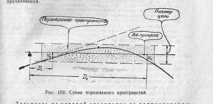
I'm working on a post about the weapons right now. RE: The accuracy values of the weapons: The DCS parameter for dispersion, Da0. Is equivalent to Range Error Probable or 0.6745. the standard deviation of dispersion (sigma). The radial dispersion values often given in western literature are also functions of the standard deviation of dispersion (sigma), assuming circular dispersion. The radius of the 80% circle is = sigma * 1.7941 As, (sqrt(-2*ln(1-0.8))) = 1.7941 To convert the DCS value of dispersion, Da0, to the 80% radius of dispersion: Da0 * (1/0.6745) * 1.7941 = The radius of 80% of the dispersion or The radius of 80% dispersion is = 2.66 * Da0. With this method we can compute the 80% radius of MIG-15 weapons in DCS and from the manual as: Projectile: DCS 80% Radius 80% Soviet Radius N-37 HEI 4.5219 2.2166 N 37 APT 4.5219 1.7733 23 mm 1.8620 3.1919 M61A1 4 50 Cal Aircraft 2.153 The increased dispersion of the 23MM cannons is probably going to improve the effectiveness of the weapons. Some dispersion is necessary to compensate for errors in fire control equipment and can reduce penalties for aiming error. To much Dispersion and the density of projectiles within the target drops. Which reduces the overall effectiveness of the system. The Soviet practice was to maximize the effectiveness of the weapons for a specific size targets over an the effective range of the weapon system. See the image below. The dispersion of the projectiles on the MiG-15 and 17 appear to optimized for their specific use cases. The 23MM being used to target fighters. The increased dispersion and rapid rate of fire would be ideal for engaging fighter sized targets at close ranges in high G maneuvering. While the 37mm would be more ideal for shooting at large non maneuvering bombers from long range.
-
Problem: The AI controlled MiG-15bis has unrealistic performance. Cause: Some of the aerodynamic characteristics of the SFM exceed those of the real aircraft. If we compare the SFM data in MiG-15bis.lua to the aerodynamic data from the real technical manual for the MiG-15bis. https://www.digitalcombatsimulator.com/en/files/2365583/ Some discrepancies are apparent. For example, the DCS MIG-15Bis SFM has 200 kgf more thrust than the real MiG-15 bis at low speed. This is because the thrust values for the SFM are based on bench tests of the VK-1 Engine and not on installed thrust data. The installation losses are given in Figure 84. The manual confirms this and notes figure 80, reflects these losses. Since thrust available defines many of the performance parameters of the aircraft. It is important that the SFM thrust parameters match this data. Using the data from the technical manual, I’ve updated almost all of the SFM of the MIG-15bis to more closely match the real aircraft. Feel free to try it out, I’ve placed a link below. The mod contains extensive notes. I cite a source for almost every change I’ve made to the SFM too. Link to Mod: https://drive.google.com/drive/folders/19cQXcBNfOdnoJkxlY2BFdUO3Zc77KESm?usp=sharing I’ve tested and validated the performance of this mod in a few different ways too. The max velocity at various altitudes, climb rates as given in table 5 of the technical manual. The SFM also matches the level acceleration data in figures 46. Below I’ll discuss some of the changes I’ve made to the SFM to more closely match the historical data below. Almost all of the aerodynamic table was changed to better match the source data. Drag: The drag polars Cx = Cx_0 + Cy^2*B2 +Cy^4*B4 Were changed to better match figures 55 and 54. A new data point was also added at mach 0.86. Which is important because the lift and drag become nonlinear here due to mach effects. LIFT: Cy max as function of Mach was changed to match Figure 185. The current values in SFM are too high, resulting in too much lift. The SFM Cy max values are drawn below in red, The mod’s Cy max are drawn in the green line. Cy Alpha was also changed to more closely match the actual aircraft. Cy0, the zero AOA lift coefficient, was set to match the lift polar in figure 51. Aldop was set to the AOA corresponding to CY max from fig 185 and Cy alpha at that mach. AOA = ((1/Cya)*Cy+((Cy0*-1)/Cya)) Engine: Some additional changes were also made to the SFM engine model. Dpdh_m was changed to more closely match the loss of thrust as a function of altitude. Thrust Kgf At Alt = Thrust Base (Kgf)-(dpdh*(Alt m*0.001) Above, the thrust available at 5000 meters for SFM is drawn in red. The mods values are drawn in blue. At low speeds the mod more closely matches real aircraft. The mod also changes to the idle rpm and thrust specific fuel to more closely data in table 19. Roll Rate: Omxmax, the max roll rate was changed to match Figure 40: Other Changes and Notes: V_opt = 367 / 3.6, -- velocity for L/D Max, Mach .3 at 0 m =367 TAS Kph Page 24 . Setting V_opt to high means the AI does not have enough excess thrust to maneuver. causing it to only do high speed loops. V_cruise = 1.31*V_opt .Def of Vopt from translation of Russian Aircraft Design book. https://archive.org/details/DTIC_AD0741485/page/62/mode/1up g_suit = 0.0, -- This Aircraft does not have a G suit, Default is 0.35, AI will sustain 6g turns all F-86 = 0.7 -- Performance Limiting Factors of AI SFM are AI Level, Cy Max, drag, Aldop, and g_suit, Vopt CAS_min = 50, -- This is Close Air Support time on station in Minutes. How long (the AI) will LOITER TIME, WEAPON CHANGES There are also some changes to the weapons parameters. I plan on doing a separate post on these changes. One of the most impactful of these changes was changing the value Tbl.effective_fire_distance to 600m to reflect the data on the 23mm and 37mm cannon uses as presented in Table 18 in The Flying Techniques and Combat Use of the MiG-17 Which gives the effective ranges when firing at fighter aircraft as 180 to 550 Meters. The previous value was 1km and resulted in a sniper bot. There are also changes to dispersion values, shell and fillers weights. These changes were made to match the data from Soviet Manual on Aircraft projectiles. https://disk.yandex.com/i/YVj0XI6O3Mu4LM That just about covers all the changes I’ve made to the MIG-15bis SFM. While these changes are not a miracle fix for the AI or the SFM. I feel the do represent a significant improvement to the AI MIG-15bis making the AI MiG-15 a much more realistic and engaging opponent. I believe this project illustrates that significant improvement to the AI performance can be made if one takes the time to realistically tune the SFM parameters. With a spreadsheet and an understanding of the SFM parameters it’s possible to create much more realistic SFM AI opponents. Eagle Dynamic could also do a lot to improve the situation by better explaining the SFM parameters. Many of the notes in various SFM files date back over a decade and are from unofficial sources, some are misleading others are simply incorrect. If you read this far, thanks for taking the time to do so. If anyone wants it, I will share the google sheet I used to help develop this MOD. Be forewarned though, it’s a hot mess and some of the units are in …Gasp! American units of insanity. I attached a track of a big dog fight mission, sabres V Mig15's down low. I know it's need for the report. Thanks for taking them time. **Updated Mod and Link to work with DCS as of July 27, 2025 MIG 15 Big Gun Fight.trk
-
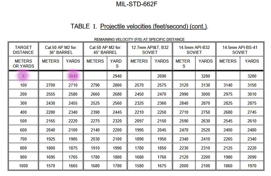
The firing table for the M8 AP is for the 28 lb 45 inch heavy barrel machine gun. The firing tables the Air Force manuals are based on the 10 lb 36 inch aircraft machine gun barrel. the reason for the difference in between the two manuals is because heavy barrel is less prone a drop in muzzle velocity than the light M2 barrel. Given the same burst length the barrel of the lighter 36 inch aircraft expands more and the overall temperature of the 36 inch barrel is greater. Resulting in a greater reduction in velocity and accuracy for the 36 inch barrel. The 28 lbs heavy barrel can fire 8 times more rounds Compared to 10 lbs 36 barrel used on aircraft machine guns. The reason for the difference in between the two manuals is because heavy barrel is less prone a drop in muzzle velocity than the light M2 barrel. If you want some direct proof that the cold barrel muzzle velocity of a 36 inch aircraft machine gun barrel firing M2 AP has a muzzle velocity of 2845 fps I'll point you to the firing tables in MIL STD 662.
- 18 replies
-
- 5
-

-

-
- investigating
- ballistics
- (and 1 more)
-
The firing tables for field use, like AAF manual 200-1, use reduced muzzle velocities for their tabulations because they are accounting for wear and the average velocity of the bullets in a burst. This is plainly stated in M8 API ballistic table. The ballistic data in those AAF field manuals. Often comes from firing tables like the one above, FT 0.5AA-T1. In “AAF-200-1 Fighter Gun Harmonization” The data comes from Aberdeen Firing Table FT. 50 AC M-1 https://archive.org/details/aaf-manual-200-1-fighter-gun-harmonization/page/9/mode/1up The ballistic data in “Air Force Manual 64 Fighter Gunnery” Comes from FT. 50 AC-M-1-8 https://archive.org/details/air-forces-manual-no.-64-fighter-gunnery-firing-rockets-dive-bombing-1-may-1945/page/111/mode/1up The reduced muzzle velocity (2700 FPS) used in AAF-200-1 is representative of a gun halfway through its service life. The Army Air Force considered a 50 caliber machine gun barrel worn out when the cold gun muzzle velocity of the weapon dropped by 200 fps. https://archive.org/details/hypervelocitygun01bush/page/466/mode/1up However, If you want some more sources with higher muzzle velocities from the war with. I can provide a few more. There’s TM 9220 It gives the muzzle for the M2 AP from the 36 inch aircraft machine guns as 2845 fps The same document gives the muzzle velocity for the M1 Incendiary when fired from the 36 inch aircraft barrel as 3,100 fps https://archive.org/details/TM9-2200/page/n209/mode/2up Or the 1944 version of “Terminal Ballistic Data” Which contains the Range, impact velocity and armor penetration values for the 50 Caliber AP M2. The test from the Ballistic Test Section was conducted on December 20 1943. This report gives the muzzle velocity of the 50 Caliber M2 AP as fired from a 36 inch aircraft barrel as 2845 fps. The 1945 Version of this same report gives the muzzle velocity as 2,835 fps. Including the data sheet. and The revised Velocity Penetration Graphic. Or From the Small arms R and D report. Which states the muzzle velocity at 78 feet from the 36 inch barrel is 2810 fps. When you take in the totality of all source materials and account for the practical application of the use of the firing table. I feel it safe to say that muzzle velocity of the 50 caliber projectiles, fired from a cold barrel, is best represented by the values in the 1946 Technical Manual for 50 Caliber aircraft Machine gun. The 2700 fps value, used in the Air Force firing tables already accounts for reduction in muzzle velocity due to burst firing and wear. When the game applies additional reductions in muzzle velocity with the shot_heat effect, it's over modeling the drop in velocity. The drop in velocity due to burst firing is baked into the Air Force firing table. The procedure for accounting for the drop in muzzle velocity due to burst fire when the firing table is created, is described by the Agency which creates those tables, The Ballistic Research Lab. In BRL Report 889 "On The Computation Procedures for Firing and Bombing Tables" https://apps.dtic.mil/sti/tr/pdf/AD0027123.pdf I know that you can ruin the performance of a 50 caliber machine gun by burst firing it. I’m not advocating for turning off shot heat for these weapons. I’m well aware that a continuous burst of 170 bullets will reduce the velocity life of a standard steel M2 50 Caliber Aircraft to zero. https://archive.org/details/hypervelocitygun01bush/page/481/mode/1up Meaning that weapon would fire 200 fps slower than a new 50 caliber, EG a worn out barrels fires around 2600 fps from a cold barrel. As this was the definition of the velocity life of the weapon. https://archive.org/details/hypervelocitygun01bush/page/466/mode/1up Velocity drop and an increase in Dispersion should be in game. However the 50 caliber machine gun DCS models is half worn out and and prone to to delivering muzzle velocities for a weapon closer to the end of its service than the begging of it . I would make this same argument for why a small reduction in the dispersion value is important. When the heat effect is added to the slightly larger dispersion, the dispersion is too great and over modeled. Again, I’m not trying to argue that burst firing should should not increase the dispersion of the projectiles. I’ve read detailed reports on how long of a burst fire it takes to reduce the accuracy of this weapon https://archive.org/details/hypervelocitygun01bush/page/466/mode/1up And The effect burst length can have on accuracy. I chose to use the 1.2 milliradian std deviation as the basis for my mod because that value is so widely used in various manuals. 4 mil 75% Shows up over and over again in numerous Air Force Weapon manuals. And It continues to show up after the war too. 4 mil 75% / 8 mil 100% was still the standard in the 1950’s https://www.google.com/books/edition/AF_Manual/81krAQAAMAAJ?hl=en&gbpv=1&pg=PA155&printsec=frontcove The fact that this figure was used over and over again for as long it did gave reasonable assurance that this was a sound basis for an accurate assessment of the gun's accuracy. There was also some other data in form of mean radius that I chose not to use because, if you computed a standard deviation for the mean radius given It was far below what the Air Force was using in their manuals. It looks like they may have had switch the notation of feet with inches when they wrote the mean radius. The document also does not define mean radius. Is it CEP? Error Probable? the Mean Radial Miss distance?. There were just to many questions about the data in this table. So I did not use any of these figures as the basis for my mod. https://archive.smallarmsreview.com/archive/detail.arc.entry.cfm?arcid=13265 I just want to impress upon you the level research and consideration that I put into developing this mod. I didn't just pick the best numbers. I selected numbers which would best represent the cold barrel performance of new 50 caliber M2 Aircraft Machine Gun. Is this the report you based your accuracy data on? Or was it that Russian P-40 firing test I've heard about but have never been able to get my hands on. I appreciate that you looked at this and I hope that I have convinced you to take another look at the data presented.
- 18 replies
-
- 4
-
-
-
- investigating
- ballistics
- (and 1 more)
-
In the hope of creating further discussion on this topic. I’ve created a “Historically Accurate 50 Cals Mod”. The mod changes the 50 caliber the muzzle velocity, projectile weight, filler weight, dispersion rating and tracer off times where appropriate, to match the historical data. This mod will only affect the aircraft and vehicles which use the WW2 50 caliber ammunition. So the P-51, P-47, ect. Aircraft, like the F-86, which use their own unique implementation of the Browning 50 caliber will not be affected by this Mod The mod is provided in a format that is compatible with the mod managers JSGME, OVGME. Using a mod manager allows you to easily toggle the mods on and off without ruining the base DCS install. Link to the Mod Below. https://drive.google.com/file/d/1dAMiOFVFmrIZQq_LtjGD-S9PsMn3z9Uz/view?usp=sharing Below is a table comparing the characteristics of the various DCS 50 caliber projectiles and those in the mod. The Mod In Detail: Due to my previous research, I’ve been able to create a mod which accurately simulates the various 50 caliber projectiles to an incredible level of detail and historical accuracy. Everything down to the tracer burn time is based on primary source materials. Below I’ll discuss all of the changes this mod makes to the various 50 caliber projectiles and provide source materials and links justifying those changes. Fair warning, things get a math heavy at the end, the dispersion section in particular. If you have any questions or comments feel free to reach out, I’m always happy to explain something. With that out of the way, let’s begin going through the changes this mod makes to the 50 caliber projectiles Muzzle Velocity: The muzzle velocity of the modded projectiles are from the 1947 version of the 50 Caliber Aircraft Machine Gun technical manual. “War Department Technical Manual, TM-9-225 Machine Gun technical manual for the Browning Machine Gun Caliber .50 AN-M2 Aircraft, Basic.” January 1947. The Manual is available on Google Books. https://books.google.com/books?id=nXySRue3QAYC&pg=PA170#v=onepage&q&f=false The muzzle velocities within this manual are the most commonly occurring values throughout the technical literature. These values are also representative of the true muzzle velocity of the bullets when being fired from the cold bore of a new gun. Therefore the muzzle velocities within the Weapon’s Technical Manual are reasonable to use as the DCS variable v0 which is equivalent to cold bore muzzle velocity in meters per second. Projectile Weight and Filler Weights: The mod changes projectile weights and payload weights of the DCS projectiles to match the weights from the projectile blueprints / schematics as presented in the Ordnance Departments Official Research Record of Small Arms and Small Arms Bullets Research and Development Report. The Official Ordnance Department’s Report is the best source for this type of information. The Ordnance Department oversaw not only weapons R and D, but also supervised the manufacture and testing of these projectiles throughout the war. The drawings / schematics of the projectiles were updated throughout the war to reflect various changes in design that occurred during the war. For example The M1 incendiary design was submitted in 1941 and was revised 10 times by 1945, the schematic was updated accordingly. Given the origin of these schematics and their continual reversion. The Ordnance Department's Report and drawings are the best source for projectile and payload weight. If you skipped down to look at the schematics, some of you may have noticed that Some of the projectile drawings have two weights listed. The M8 API for example During the war, the Tungsten Chromium core was replaced with a lower weight hardened steel core. page 190 of the Army Ordnance Research and Development Report for Small Arms Ammunition. 1946. https://archive.smallarmsreview.com/archive/detail.arc.entry.cfm?arcid=13268 Therefore the weights of the Modded projectiles are equal to those of Alternate core versions. As the alternate core 50 caliber ammunition would have been in use during World War 2. Below, In the spoilers, are the blueprints for the 50 Caliber Projectiles effected by this mod. The design drawings all come from various parts of the “Army Ordnance Small Arms Ammunition Development Report” The only link I can provide to this document is from The Archive of the Small Arms Review. The report is split into 6 parts, all of which can be downloaded for free. Link to Part 1: https://archive.smallarmsreview.com/archive/detail.arc.entry.cfm?arcid=13265 Blueprint M2 AP Blueprint M8 API Blueprint M20 APIT Blueprint M1 Incendiary Blueprint M1 Tracer The weight of the incendiary payload in the mod, is equal to the weight of the incendiary payload + half the weight of tracer composition. The M 20 APIT has a payload of 18 grains of incendiary and contains 14 grains of tracer. Thus the payload of the M 20 APIT in the mod is 25 grains, as 18 + (14*0.5) = 25 grains or 0.0016 kilograms. Tracer Burn Times: For the M1 Tracer, burn time is directly from from The Ordnance R and D report. The M1 Tracer burns for 3.8 seconds. Therefore, the mod sets the tracer off time to 3.8 seconds for the M1 Tracer. Determining the appropriate trace off time for the M20 APIT is a bit more complicated. As I could not find an exact tracer burn out time for the M20 APIT, only the specified burn distance. So we’ll have to compute the time of flight to burn out distance. Warning there be maths below! The Ordnance Department’s Research And Development Report on Small Arms Ammunition Tracers does give the length of tracer burn. The Tracer is expected to burn over 1800 yards. https://archive.smallarmsreview.com/archive/detail.arc.entry.cfm?arcid=13266 A footnote in M2 50 Caliber Machine Gun’s technical manual gives a similar burn out distance. In DCS we specify the burn out time of the tracer. If we want the mod to match the historical data, we just have to compute the TOF of M20 APIT to 1800 yards. Then set the tracer on M20 APIT to turn off when the bullet has flown 1800 yards. As the goal of this mod is historical accuracy. When we compute the time of flight to 1800 yards, We’ll use the same methodology the Ballistic Research Laboratory employed to compute firing tables during World War 2. This computed TOF to 1800 yards will be the number of seconds DCS waits before turning off the tracer effect. The analytical technique used to compute firing / ballistic tables is explained in detail within the National Defense Research Committee report “Analytical Studies in Aerial Warfare”. https://archive.org/details/analyticalstudie02bush/page/12/mode/1up Putting the time of flight equation into something a bit more manageable we get. TOF= (1/((V0/Range)-((.00372*rho)/(2*BC)*Sqrt(V0))) Where V0 = The Bullets Muzzle Velocity + The Aircraft Speed (TAS) In FPS, We’ll set V0 to the muzzle velocity of M20 APIT, when being fired from a stationary position on the ground, from an M2 machine gun with a 36 inch aircraft barrel. The Technical Manual for the 50 Caliber M2 Caliber Aircraft Machine gives the muzzle velocity of M20 APIT as 2950 fps. V0= 2950 (fps) C5 is the C5 ballistic coefficient of 50 Caliber M20 APIT, This value is = 0.437 As is stated in BRL Report Form Factors of Projectiles. https://apps.dtic.mil/sti/pdfs/AD0802080.pdf C5 = 0.437 Rho is the relative air density to the sea level standard ballistic density 0.07513 lb / feet^3. This is also called the density ratio. At sea level, on a standard day, this value is 1. Rho =1 The Range is 1800 yards, however this equation uses feet as the format for the range input. So we just convert yards to feet and Range is set to. Range = (1800*3) The NDRC equation configured to compute the TOF to 1800 yards for the M20 APIT now looks like: TOF = (1/((2950/(1800*3))-((.00372*1)/(2*0.437)*Sqrt(2950))) Thus TOF To 1800 Yards = 3.173390047 Seconds. Let's compare our computed TOF to some historical data and see if the NDRC time of flight equation we used is accurate. We’ll look at a Ballistic table for the M8 API from 1946. Given that, the M8 API is a ballistic match to the M20 APIT . if we correctly set up the NDRC TOF equation and compute the TOF of the M8 API to 1800. And, the computed TOF is equal to the TOF data within the real Ballistic / Firing table. We can reasonably assume that the computed TOF of the M20 APIT is accurate. This Firing table is for an M8 API fired from a 45 inch heavy barrel version of the 50 Caliber Browning, with a muzzle velocity of 3000 fps The ballistic table says the time of flight to 1800 yards is 3.08 seconds. Now we just have to configure the NDRC TOF equation with the proper variables for the M8 API. If the computed time of flight to 1800 yards is close to 3.08 we can assume this equation is accurate enough for our mod. To configure the TOF equation to compute the TOF of M8 API to 1800 yards. We change the muzzle velocity to be equal to the muzzle velocity in the ballistic table. Meaning we set V0, to 3000 fps V0 =3000, We also have to change the C5 ballistic coefficient the correct value for the M8 API, which is 0.439 https://apps.dtic.mil/sti/pdfs/AD0491936.pdf BC M8 API = 0.439 The range is still = (1800*3) feet The time of flight equation for the M8 API to 1800 yards is now: TOF Computed M8 API = (1/((3000/(1800*3))-((0.00372*1)/(2*0.439)*Sqrt(3000)))) TOF Computed M8 API = 3.091277324 Seconds The computed TOF to 1800 yards is 3.09127 seconds. The TOF for M8 API using the NDRC equation is 3.09 seconds. In the real ballistic table the TOF to 1800 yards is 3.08 seconds. The computed TOF is 0.01 seconds longer. A difference of +0.0032%. The high level of accuracy of the NDRC method means that it can be relied upon to compute the TOF M20 APIT to 1800 yards. Based upon the accuracy of NDRC method I’ve set the tracer off time of the M20 APIT to 3.1 seconds. Dispersion Data: The variable DCS uses to describe the weapon dispersion is Da0. In the Western technical literature this variable is equivalent to Deflection Error Probable or Range Error Probable. Error Probable is equal to 0.6745 * the standard deviation of dispersion from the aim point in the x or y axis alone. https://apps.dtic.mil/sti/tr/pdf/AD1009077.pdf Error Probable as a measure of accuracy is more commonly used in Soviet and Russian sources. The Image in the spoiler Below is from a manual on Soviet Aircraft Ammunition from the 1950’s. The Manual gives the error probable for few Soviet Cold War Era aircraft cannons in meters. On the other hand, Western Sources often depict accuracy as the radius or diameter of a circle and a percentage. For example, the 1945 “Air Force Gunnery Manual 64” states the dispersion of the 50 Caliber Browning is a diameter of 4 mils 75%. https://archive.org/details/air-forces-manual-no.-64-fighter-gunnery-firing-rockets-dive-bombing-1-may-1945/page/67/mode/1up To convert the Western accuracy measurement, a diameter of 4 mil 75%, to the same format as DCS uses (Error Probable) we have to do some math. First, We’re going to use the 4 mil 75% accuracy rating of the 50 Caliber and determine the standard deviation of the dispersion, also known as sigma. After, we have determined sigma. It’s relatively easy to convert sigma to Error Probable, then convert Error probable from mils to radians, which is the format DCS uses for the accuracy rating Da0. The value 4 Mil 75% is a function of a circular bivariate normal distribution. The diameter of a circle containing a given probability is = The standard deviation of the distribution of the dispersion (sigma) * sqrt(-8*ln(1-the probability of the circle). Therefore, the diameter of 75% circle is equal to: Sigma * sqrt(-8*ln(1-0.75) = The Diameter of 75% Circle Which simplifies to: Sigma * 3.33021 = The Diameter of 75% Circle Since the document gives us the diameter of the circle (4 mils). We know that: Sigma * 3.33021 = 4 With some simple algebra, we can now determine sigma. By dividing 4 mils / 3.33021 we get sigma 4/3.33021 = sigma = 1.2011 mils Our computed value of sigma agrees with other values of sigma present in the technical literature. Standard Deviation Source. From “Analytical Studies in Aerial Warfare” https://archive.org/details/analyticalstudie02bush/page/105/mode/1up Now that we have sigma, all we have to do is convert sigma to Error Probable. Which is pretty straight forward. Sigma * 0.6745 = Error Probable (Mils) 1.2011*0.6745 = 0.810 Error Probable (Mils) The variable for dispersion in DCS, Da0, is in radians, To convert mils to radians. Multiply by 0.001 Thus Da0 50 Cal Mod = 0.810 *0.001 Da0 50 Cal Mod = 0.00081. The current value of Da0 for the 50 Cal is = 0.00085, Which equates to a standard deviation of 1.26 Mils. The standard deviation of the 50 Cal Mod is 1.2 mils. The net result of the mod is a 10% reduction in area of Circle Error Probable. In the web based graphing application Desmos. I’ve created a simulation that randomly places some random normally distributed "bullet impacts." While plotting the Circle Error Probable aka the 50% impact circle of dispersion. Link to the Dispersion Sim https://www.desmos.com/calculator/srjak2emph With this tool we can easily create an accurate depiction of the Modded Dispersion, which has a 1.41 Mils 50% radius. Thus the radius of Circle Error Probable for the Mod is 1.41 Mils. And the radius of 50 % percent circle / Circle Error Probable for the default DCS World War 2 50 caliber Projectiles is 1.48 mils. Yeah that was a lot of math for not much of a change in dispersion. The size of the dispersion in DCS before barrel heat effects are applied is only slightly off. However, this small change does make the bullets more historically accurate, which is the intent of this mod. While we did not end up with large change to the dispersion. I did learn a lot from research that went into determining the appropriate value of Da0. I ended up with a much better understanding of how the accuracy values of the weapons in DCS relate to the real world accuracy ratings. This knowledge will end up helping me with a few other projects I have in mind too. With the dispersion taken care of, we have just about covered all the changes this mod makes to the 50 caliber projectiles. However we do have a few miscellaneous changes to cover Other Changes and Final Notes: DCS also has a variable which randomizes the muzzle velocity of the project, Dv0. This is set to 0 in the mod during test and validation and has been left off. The duration of the smoke effect has been reduced. In DCS the Smoke effect of the tracer effect doesn’t match the trajectory of the bullet. The smoke effect just travels straight out from the gun barrel. Thus the smoke tends to hinder aiming. The thickness and amount of smoke produced by the effect also obscures the visual signature of the tracer glow. Which also greatly reduces the effectiveness of the tracer as an aiming aid. Thus the smoke time has been reduced from 0.5 Seconds to 0.1 Seconds. I’ve also changed the projectile type of the M1 Incendiary from Ball to AP. The M1 Incendiary was manufactured around a tubular steel dowel / frame. The thick steel sleeve and high muzzle velocity gave the M1 Incendiary the ability to penetrate armor up to 7/8 inches thick. This excerpt is from the US Army Air Forces Aircraft Evaluation Report of The Messerschmitt -109F Link to the 109F report: https://stephentaylorhistorian.files.wordpress.com/2020/04/bf-109f-evaluation.pdf Given the M1-Inc’s ability to penetrate fairly thick armor, the change in projectile type is reasonable. That covers all the changes this mod makes to DCS 50 caliber projectiles. If you have read this far down I want to thank you for taking the time to do so. If you have any questions please feel free to ask. I’m always happy to help.
- 18 replies
-
- 6
-
-
-
- investigating
- ballistics
- (and 1 more)
-
I found the source for the DCS pattern. It's from the North American Aviation Version of the flight Manual. https://app.aircorpslibrary.com/document/viewer/fmp51na5914 The pattern. The DCS pattern is an almost exact fit of this pattern. The NAA manual pattern being the dashed lines. https://www.desmos.com/calculator/2dnjxa31ca It does look like someone from NAA may have miss interpreted the Air Force pattern. As the NAA pattern also mirrors the dispersion pattern. https://www.desmos.com/calculator/ngk08zcyuh And the NAA pattern Disappears from all the documents published after this manual. NAA Harmonization / Convergence Pattern K-14 Sight NAA Manual Azimuth Azimuth Degrees Elevation Elevation Degrees Gun 1 72.5 38.375 0.006623 0.3794699477 0.006348 0.3637136083 Gun 2 82.08823529 36 0.005002764706 0.2866373035 0.007493 0.4293172759 Gun 3 89.125 39 0.005951 0.3409671839 0.005002 0.2865934891